AI/ML Cheatsheet

2.1 Linear Algebra

• Linear Algebra deals with numbers organized in arrays and how these arrays interact. It is used in almost every ML algorithm.

2.1.1 Vectors, Matrices, and Tensors

• Vector: A 1D array of numbers. Example: $[3, 5, 7]$
• Used to represent features like height, weight, age.
• Matrix: A 2D array (rows and columns).
• Example:

  
  [[2,4],
  [6,8]]
                                      

• Used to store datasets or model weights.
• Tensor: A generalization of vectors and matrices to more dimensions (3D or higher).
• Example: Used in deep learning models like images (3D tensor: width, height, color channels).

2.1.2 Matrix Operations

• Addition/Subtraction: Add or subtract corresponding elements of two matrices.
• Multiplication: Used to combine weights and inputs in ML models.
• Transpose: Flip a matrix over its diagonal.
• Dot Product: Fundamental in calculating output in neural networks.

2.1.3 Eigenvalues and Eigenvectors

• Eigenvector: A direction that doesn't change during a transformation.
• Eigenvalue: Tells how much the eigenvector is stretched or shrunk.

These are used in algorithms like Principal Component Analysis (PCA) for dimensionality reduction.

2.2 Probability and Statistics

Probability helps machines make decisions under uncertainty, and statistics helps us understand data and model performance.

2.2.1 Mean, Variance, Standard Deviation

• Mean: The average value.
• Variance: How spread out the values are from the mean.
• Standard Deviation: The square root of variance. It measures how much the values vary.

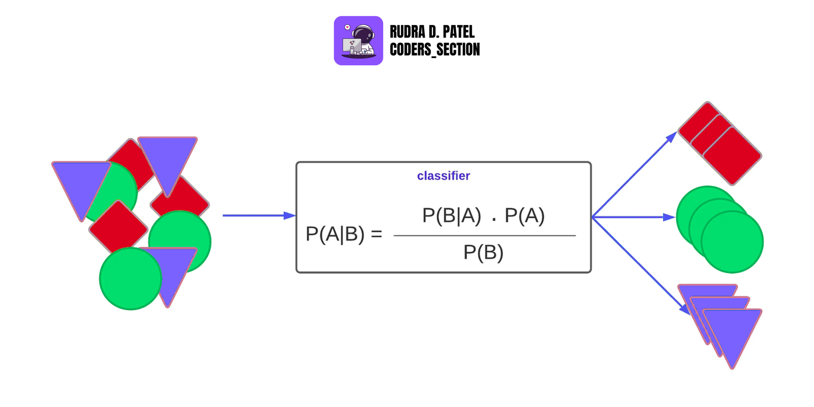
2.2.2 Bayes Theorem

Formula: $P(A|B) = \frac{P(B|A) \cdot P(A)}{P(B)}$

Used in Naive Bayes classifiers for spam detection, document classification, etc.

2.2.3 Conditional Probability

The probability of one event occurring given that another event has already occurred.

Example:

• Probability that a user clicks an ad given that they are between 20-30 years old.

2.2.4 Probability Distributions

• Normal Distribution: Bell-shaped curve. Common in real-world data like height, exam scores.
• Binomial Distribution: Used for yes/no type outcomes. Example: Flipping a coin 10 times.
• Poisson Distribution: For events happening over a time period. Example: Number of customer calls per hour.

These distributions help in modeling randomness in data.

2.3 Calculus for Optimization

Calculus helps in training models by optimizing them to reduce errors.

2.3.1 Derivatives and Gradients

• Derivative: Measures how a function changes as its input changes.
• Gradient: A vector of derivatives that tells the slope of a function in multi dimensions.

Used to find the direction in which the model should adjust its weights.

2.3.2 Gradient Descent

• An optimization algorithm used to minimize the loss (error) function.

How it works:

• Start with random values
• Calculate the gradient (slope)
• Move slightly in the opposite direction of the gradient
• Repeat until the loss is minimized

Gradient Descent is the core of many training algorithms in ML and DL.

3.1 Data Cleaning

Real-world data is often messy. Data cleaning means identifying and fixing errors in the dataset.

3.1.1 Missing Values

Missing values can be due to incomplete forms, sensor errors, etc.

Techniques to handle missing data:

• Remove rows/columns with too many missing values
• Fill (impute) missing values using:
• Mean/Median/Mode
• Forward/Backward fill
• Predictive models (like KNN)

3.1.2 Outliers

Outliers are data points that are very different from others.

They can distort results and reduce model performance.

Detection methods:

• Box plot, Z-score, IQR method

Handling outliers:

• Remove them
• Transform data (e.g., log scaling)
• Cap them (set a maximum/minimum)

3.2 Data Normalization and Standardization

Helps scale numeric data so that features contribute equally to the model.

Normalization (Min-Max Scaling):

Formula: $X_{normalized} = \frac{X - X_{min}}{X_{max} - X_{min}}$

Standardization (Z-score Scaling):

Formula: $X_{standardized} = \frac{X - \mu}{\sigma}$

3.3 Encoding Categorical Variables

ML models work with numbers, not text. Categorical data needs to be converted into numerical form.

Label Encoding:

Assigns each unique category a number.

One-Hot Encoding:

Creates new binary columns for each category.

Label encoding is good for ordinal data (ranked), while one-hot encoding is best for nominal data (non-ranked).

3.4 Feature Scaling

Ensures features are on the same scale so the model can learn effectively.

• Min-Max Scaling:
• Scales features between 0 and 1.
• Good for algorithms like KNN, neural networks.
• Z-score Scaling (Standardization):
• Useful for models that assume normality, like linear regression or logistic regression.

Scaling is crucial for models that use distance or gradient-based optimization.

3.5 Feature Engineering

Creating new features or modifying existing ones to improve model performance.

• Polynomial Features:
• Create new features by raising existing features to a power.
• Example: From x, create $x^2, x^3$
• Binning (Discretization):
• Grouping continuous values into bins or intervals.
• Example: Age (0-10, 11-20, etc.)

3.6 Handling Imbalanced Data

In classification, if one class dominates (e.g., 95% non-fraud, 5% fraud), models may ignore the minority class. This is called class imbalance.

• SMOTE (Synthetic Minority Oversampling Technique):
• Creates synthetic examples of the minority class using nearest neighbors.
• Undersampling:
• Remove some samples from the majority class.
• Oversampling:
• Duplicate or generate more samples of the minority class.

Balancing data improves the ability of the model to correctly predict both classes.

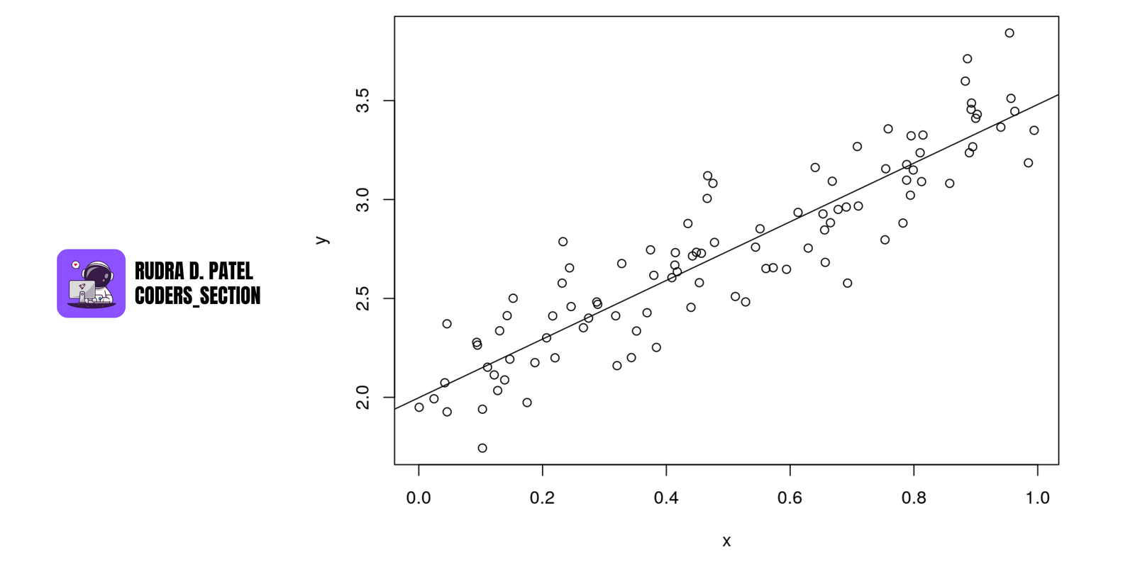
4.1 Linear Regression

Used for predicting continuous values (e.g., predicting house price, temperature).

4.1.1 Simple vs. Multiple Linear Regression

• Simple Linear Regression: One input (X) to predict one output (Y).
• Example: Predicting salary from years of experience.
• Multiple Linear Regression: Multiple inputs ($X_1, X_2, ..., X_n$).
• Example: Predicting price based on area, location, and age.

4.1.2 Gradient Descent and Normal Equation

• Gradient Descent: Iterative method to minimize error (cost function).
• Normal Equation: Direct way to find weights using linear algebra.

$\theta = (X^T X)^{-1} X^T y$

Works for small datasets.

4.1.3 Regularization (L1, L2)

Prevents overfitting by adding a penalty:

• L1 (Lasso): Can reduce coefficients to 0 (feature selection).
• L2 (Ridge): Shrinks coefficients but doesn’t make them 0.

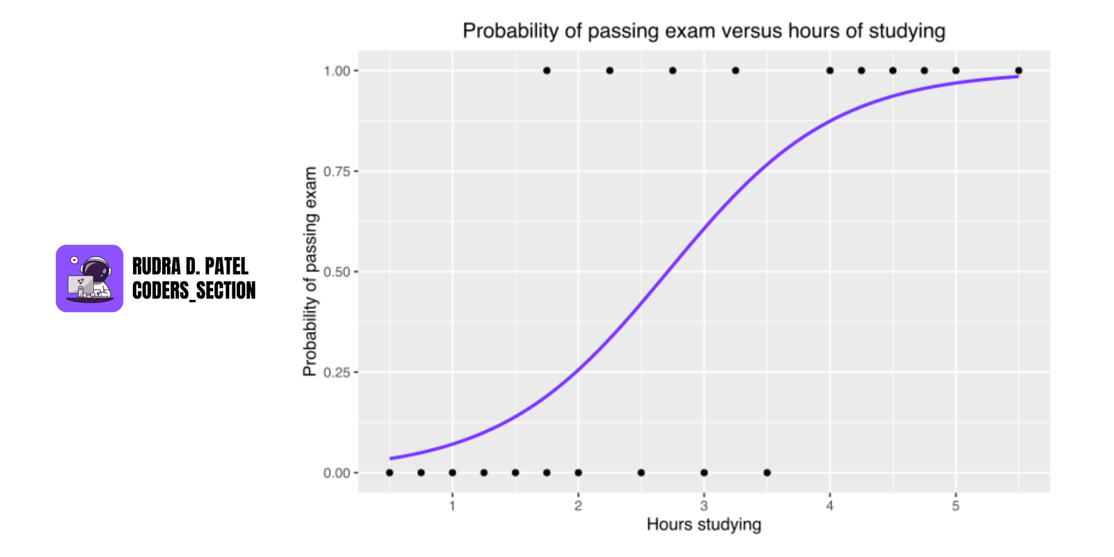
4.2 Logistic Regression

Used for classification problems (e.g., spam vs. not spam).

4.2.1 Binary vs. Multiclass Classification

• Binary: 2 outcomes (e.g., 0 or 1)
• Multiclass: More than 2 classes (handled using One-vs-Rest or Softmax)

4.2.2 Sigmoid and Cost Function

• Sigmoid Function: Converts outputs to values between 0 and 1.

• Cost Function: Log loss used to measure prediction error.

4.2.3 Regularization

• L1 and L2 regularization help prevent overfitting in logistic regression as well.

4.3 K-Nearest Neighbors (KNN)

A simple classification (or regression) algorithm that uses proximity.

4.3.1 Distance Metrics

• Euclidean Distance: Straight line between two points.
• Manhattan Distance: Sum of absolute differences.

4.3.2 Choosing K

• K is the number of neighbors to consider.
• Too low K → sensitive to noise
• Too high K → model becomes less flexible

4.3.3 Advantages & Disadvantages

• Simple and easy to implement
• Slow for large datasets, sensitive to irrelevant features

4.4 Support Vector Machines (SVM)

Powerful classification model for small to medium-sized datasets.

4.4.1 Hyperplanes and Margins

• SVM finds the best hyperplane that separates data with maximum margin.

4.4.2 Linear vs. Non-Linear SVM

• Linear SVM: Works when data is linearly separable.
• Non-linear SVM: Uses kernel trick for complex datasets.

4.4.3 Kernel Trick

• Transforms data into higher dimensions to make it separable.
• Common kernels: RBF (Gaussian), Polynomial, Sigmoid

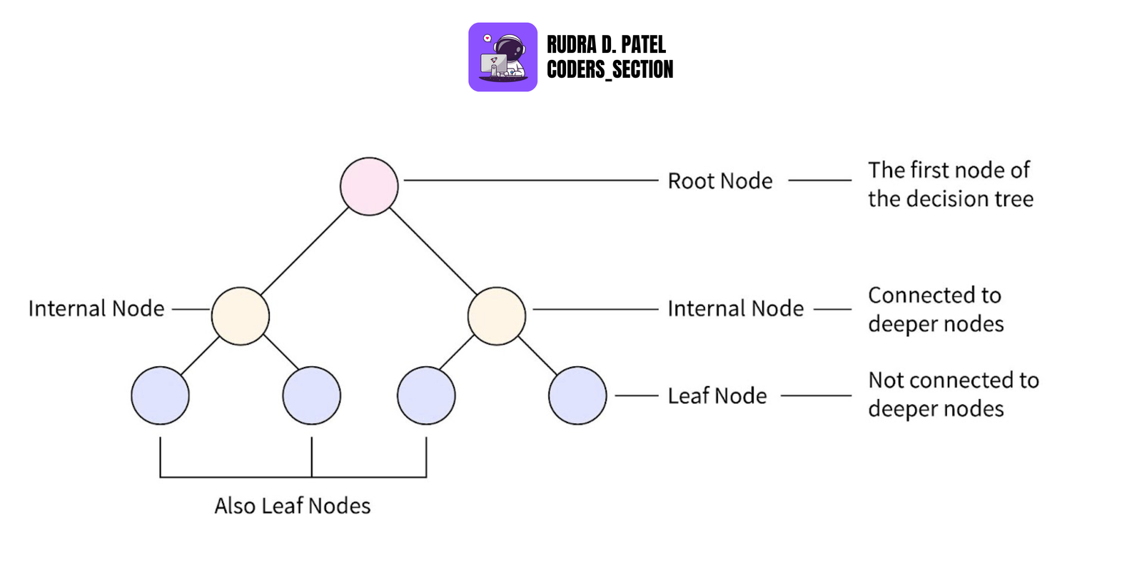
4.5 Decision Trees

Tree-like structure used for classification and regression.

4.5.1 Gini Impurity and Entropy

Measures how pure a node is:

• Gini Impurity: Probability of misclassification.
• Entropy: Measure of randomness/information.

4.5.2 Overfitting and Pruning

• Overfitting: Tree memorizes training data.
• Pruning: Removes unnecessary branches to reduce overfitting.

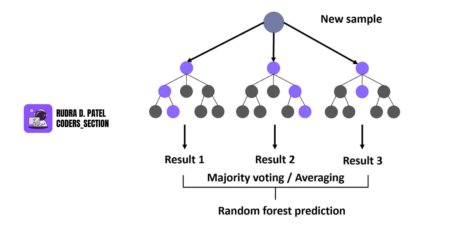
4.6 Random Forest

An ensemble of decision trees to improve accuracy and reduce overfitting.

4.6.1 Bootstrapping

• Randomly selects subsets of data to train each tree.

4.6.2 Bagging

• Combines predictions of multiple trees (majority vote or average).

4.6.3 Feature Importance

• Measures which features contribute most to model prediction.

4.7 Gradient Boosting Machines (GBM)

Boosting is an ensemble method where models are trained sequentially.

4.7.1 XGBoost, LightGBM, CatBoost

Advanced boosting libraries:

• XGBoost: Popular, fast, and accurate
• LightGBM: Faster, uses leaf-wise growth
• CatBoost: Handles categorical features automatically

4.7.2 Hyperparameter Tuning

Adjust parameters like:

• Learning rate
• Number of estimators (trees)
• Max depth

Tools: GridSearchCV, RandomSearchCV

4.7.3 Early Stopping

• Stops training if the model stops improving on validation set.

4.8 Naive Bayes

Probabilistic classifier based on Bayes' Theorem and strong independence assumption.

4.8.1 Gaussian, Multinomial, Bernoulli

• Gaussian NB: For continuous features (assumes normal distribution)
• Multinomial NB: For text data, counts of words
• Bernoulli NB: For binary features (0/1)

4.8.2 Assumptions and Applications

• Assumes all features are independent (rarely true but still works well)
• Commonly used in spam detection, sentiment analysis, document classification

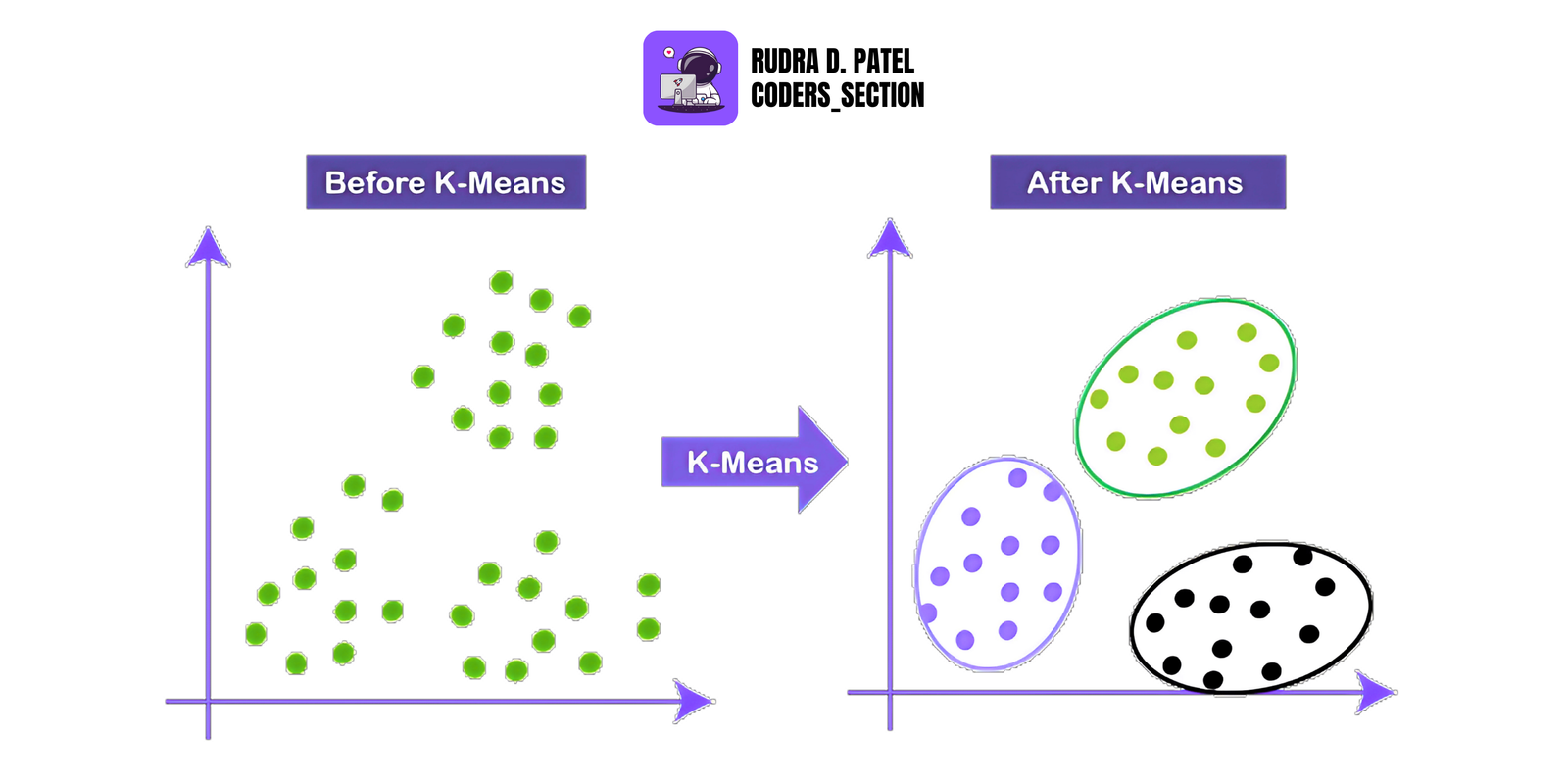
5.1 K-Means Clustering

5.1.1 Algorithm Overview

K-Means is a clustering algorithm that divides data into K clusters based on similarity.

It works by:

1. Selecting K random centroids.
2. Assigning each point to the nearest centroid.
3. Updating the centroid to the mean of its assigned points.
4. Repeating steps 2–3 until the centroids stop changing.

5.1.2 Elbow Method

• Used to choose the optimal number of clusters (K).
• Plot the number of clusters (K) vs. Within-Cluster-Sum-of-Squares (WCSS).
• The point where the WCSS curve bends (elbow) is the best K.

5.1.3 K-Means++ Initialization

• Improves basic K-Means by smartly selecting initial centroids, reducing the chance of poor clustering.
• Starts with one random centroid, then selects the next ones based on distance from the current ones (probabilistically).

5.2 Hierarchical Clustering

5.2.1 Agglomerative vs. Divisive Clustering

• Agglomerative (bottom-up): Start with each point as its own cluster and merge the closest clusters.
• Divisive (top-down): Start with one large cluster and recursively split it.

Agglomerative is more commonly used.

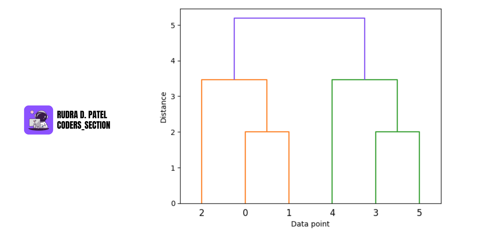
5.2.2 Dendrogram and Optimal Cut

• A dendrogram is a tree-like diagram that shows how clusters are formed at each step.
• The height of branches represents the distance between clusters.
• Cutting the dendrogram at a certain height gives the desired number of clusters.

5.3 Principal Component Analysis (PCA)

PCA is a dimensionality reduction technique used to simplify datasets while retaining most of the important information.

5.3.1 Dimensionality Reduction

• PCA transforms the data into a new coordinate system with fewer dimensions (called principal components).
• Useful for visualization, speeding up algorithms, and avoiding the curse of dimensionality.

5.3.2 Eigenvalue Decomposition

• PCA is based on eigenvectors and eigenvalues of the covariance matrix of the data.
• The eigenvalues indicate the amount of variance explained by each principal component.

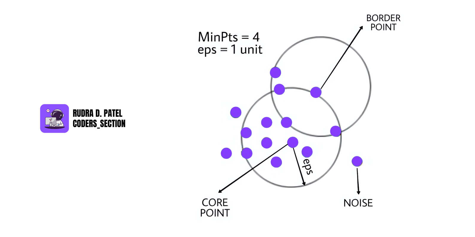
5.4 DBSCAN (Density-Based Spatial Clustering of Applications with Noise)

DBSCAN is a density-based clustering algorithm that groups closely packed points and marks outliers as noise.

5.4.1 Density-Based Clustering

• Unlike K-Means, DBSCAN doesn't require specifying the number of clusters.
• Clusters are formed based on dense regions in the data.

5.4.2 Epsilon and MinPts Parameters

• Epsilon ($\epsilon$): Radius around a point to search for neighbors.
• MinPts: Minimum number of points required to form a dense region.

Points are classified as:

• Core Point: Has MinPts within $\epsilon$.
• Border Point: Not a core but within $\epsilon$ of a core.
• Noise: Neither core nor border.

6.1 Introduction to Reinforcement Learning

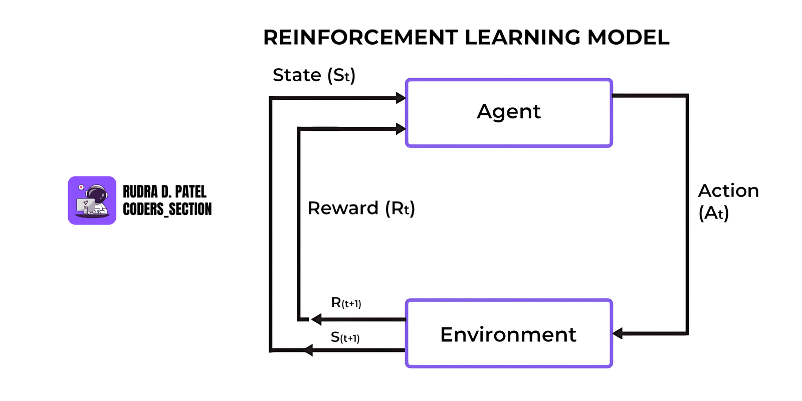
6.2 Key Concepts

• Agent: The learner or decision maker (e.g., a robot, self-driving car).
• Environment: Everything the agent interacts with (e.g., a maze, a game).
• State: A snapshot of the current situation (e.g., position in a maze).
• Action: A move or decision made by the agent (e.g., turn left).
• Reward: Feedback from the environment (e.g., +1 for reaching goal, -1 for hitting a wall).

The goal of the agent is to maximize cumulative rewards over time.

6.3 Markov Decision Process (MDP)

• RL problems are often modeled as Markov Decision Processes (MDPs).

An MDP includes:

• S: Set of states
• A: Set of actions
• P: Transition probabilities ($P(s' | s, a)$)
• R: Reward function
• $\gamma$ (gamma): Discount factor (how much future rewards are valued)

The "Markov" property means the next state only depends on the current state and action, not on previous ones.

6.4 Q-Learning and Deep Q-Networks (DQN)

Q-Learning:

• A model-free algorithm that learns the value (Q-value) of taking an action in a state.
• Uses the formula:

$Q(s, a) = Q(s, a) + \alpha [r + \gamma \max_{a'} Q(s', a') - Q(s, a)]$

Where:

• s: current state
• a: action
• r: reward
• s': next state
• $\alpha$: learning rate
• $\gamma$: discount factor

Deep Q-Networks (DQN):

• When the state/action space is too large, a neural network is used to approximate Q-values.
• Combines Q-Learning with Deep Learning.
• Used in Atari games and robotics.

6.5 Policy Gradients and Actor-Critic Methods

Policy Gradients:

• Instead of learning value functions, learn the policy directly (probability distribution over actions).
• Use gradient ascent to improve the policy based on the reward received.

Actor-Critic Methods:

• Combine the best of both worlds:
• Actor: chooses the action
• Critic: evaluates how good the action was (value function)
• More stable and efficient than pure policy gradients.

6.6 Exploration vs. Exploitation

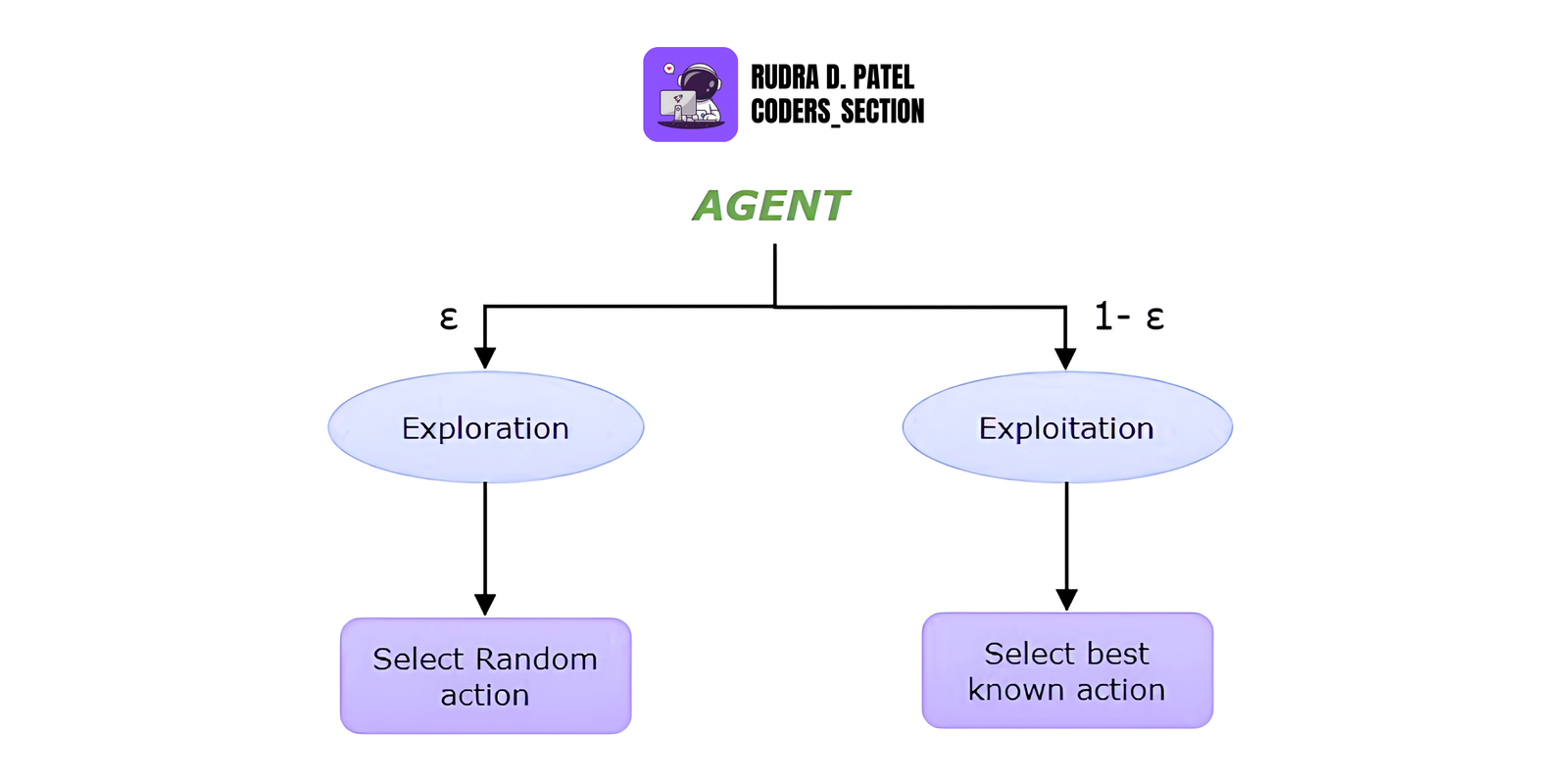
• Exploration: Trying new actions to discover their effects (important early in training).
• Exploitation: Choosing the best-known action for maximum reward.

RL must balance both:

• Too much exploration = slow learning
• Too much exploitation = stuck in local optimum

Common strategy: $\epsilon$-greedy

• Choose a random action with probability $\epsilon$
• Otherwise, choose the best-known action

7.1 Introduction to Neural Networks

A neural network is a computer model inspired by the human brain. It consists of neurons (nodes) organized in layers, capable of learning patterns from data.

7.1.1 Perceptrons

The perceptron is the simplest type of neural network, with:

• Inputs → Weights → Summation → Activation Function → Output

It's like a yes/no decision maker (binary classification).

7.1.2 Activation Functions

These introduce non-linearity, allowing the network to learn complex functions:

• Sigmoid: Outputs between 0 and 1. Good for probability-based outputs.
• ReLU (Rectified Linear Unit): Most popular. Fast, reduces vanishing gradient.
• ReLU(x) = $\max(0, x)$
• Tanh: Like sigmoid but outputs between -1 and 1.

7.1.3 Forward Propagation and Backpropagation

• Forward Propagation: Input data flows through the network to produce an output.
• Backpropagation: Calculates the error and updates weights using gradients (from loss function).

This is how neural networks learn from data.

7.1.4 Loss Functions

They measure how far off the model's predictions are from the actual values.

• MSE (Mean Squared Error): For regression.
• Cross-Entropy: For classification.

7.2 Deep Neural Networks (DNN)

7.2.1 Architecture and Layers

• Input Layer: Where the data comes in
• Hidden Layers: Where computation happens (many neurons per layer)
• Output Layer: Final predictions

7.2.2 Training Process and Optimizers

During training, the network:

• Makes predictions
• Calculates the loss
• Updates weights via optimizers like:
• SGD (Stochastic Gradient Descent)
• Adam (adaptive learning rate)
• RMSProp

7.2.3 Overfitting and Regularization

Overfitting happens when the model learns noise instead of patterns.

Regularization techniques help:

• Dropout: Randomly turns off neurons during training.
• L2 Regularization: Penalizes large weights (weight decay).

7.3 Convolutional Neural Networks (CNN)

CNNs are specialized for image data.

7.3.1 Convolutional Layers, Pooling Layers

• Convolutional Layers: Apply filters to detect features (edges, corners).
• Pooling Layers: Reduce size of feature maps (e.g., Max Pooling).

7.3.2 Filters/Kernels and Strides

• Filters: Small matrix to slide over input to extract features.
• Strides: How many steps the filter moves.

7.3.3 Applications (Image Classification, Object Detection)

• Image Classification: Categorizing images (e.g., cat or dog).
• Object Detection: Finding and locating objects in an image.

7.4 Recurrent Neural Networks (RNN)

RNNs are designed for sequential data (time series, text, etc.).

7.4.1 Basic RNN vs. LSTM vs. GRU

• Basic RNN: Loops through time steps but suffers from memory issues.
• LSTM (Long Short-Term Memory): Handles long dependencies well.
• GRU (Gated Recurrent Unit): Similar to LSTM but faster.

7.4.2 Time-Series Prediction and NLP Applications

• Predict stock prices, weather, or language sequences.
• Used in chatbots, translation, and speech recognition.

7.4.3 Vanishing and Exploding Gradients Problem

• Problem during training of RNNs where gradients shrink (vanish) or explode.
• LSTM and GRU solve this with gate mechanisms.

7.5 Generative Adversarial Networks (GANs)

GANs are powerful models for generating new data.

7.5.1 Generator and Discriminator

• Generator: Creates fake data
• Discriminator: Tries to distinguish real from fake data

They compete with each other (like a forger and a detective).

7.5.2 Training Process

• Generator tries to fool the discriminator
• Discriminator improves to detect fakes
• They both improve over time — leading to realistic generated data

7.5.3 Applications

• Image Generation (e.g., fake faces)
• Art and Style Transfer
• Data Augmentation for training other ML models

8.1 Text Preprocessing

Before using text in machine learning models, we need to clean and convert it into a format the computer understands.

• Tokenization:
• Breaking text into smaller parts like words or sentences.
• Example: "I love AI" → ["I", "love", "AI"]
• Stopwords:
• Removing common words that do not add much meaning (like “is”, “the”, “and”).
• Stemming:
• Cutting words down to their root form.
• Example: “playing”, “played” → “play”
• Lemmatization:
• Similar to stemming but uses grammar to find the proper base word.
• Example: “better” → “good”
• Bag of Words (BoW):
• Converts text into numbers based on word counts in a document.
• TF-IDF:
• Gives importance to words that appear often in one document but not in others. Helps identify keywords.

8.2 Word Embeddings

Word embeddings turn words into vectors (numbers) so that a machine can understand their meaning and context.

• Word2Vec:
• A model that learns how words are related based on their surrounding words.
• GloVe:
• Learns word meanings by looking at how often words appear together.
• FastText:
• Similar to Word2Vec but also looks at parts of words, which helps with unknown words.
• Sentence Embeddings (BERT, RoBERTa, GPT):
• These models convert full sentences into vectors. They understand context much better than older models.

8.3 Sequence Models

These models are good for processing data where order matters, like text.

• RNN (Recurrent Neural Networks):
• Good for learning from sequences, such as sentences.
• LSTM (Long Short-Term Memory):
• An advanced RNN that remembers long-term information.
• GRU (Gated Recurrent Unit):
• A simpler version of LSTM that works faster and often just as well.

8.4 Transformer Architecture

Transformers are a powerful modern architecture, especially for NLP tasks, known for their ability to process sequences in parallel and capture long-range dependencies using attention mechanisms.

• Self-Attention Mechanism:
• Allows the model to weigh the importance of different words in the input sequence when processing each word.
• Encoder-Decoder Model:
• Encoders process the input sequence, and decoders generate the output sequence.
• BERT, GPT, T5 Models:
• Popular transformer-based models for various NLP tasks.

8.5 Text Classification

Classify text into categories.

Examples:

• Sentiment Analysis: Is a review positive or negative?
• Named Entity Recognition (NER): Find names, places, dates, etc. in text.

8.6 Language Generation

Generate new text from existing input.

8.6.1 Text Summarization

• Shortens a long document while keeping important points.

8.6.2 Machine Translation

• Translates text from one language to another (like English to Hindi).

9.1 Classification Metrics

Used when your model predicts categories or classes (e.g., spam or not spam).

9.1.1 Accuracy

• How often the model is correct.
• Formula: $\frac{\text{Correct Predictions}}{\text{Total Predictions}}$

9.1.2 Precision

• Out of all predicted positives, how many were actually positive?
• Used when false positives are costly.
• Formula: $\frac{\text{TP}}{\text{TP + FP}}$

9.1.3 Recall (Sensitivity)

• Out of all actual positives, how many were predicted correctly?
• Used when missing positives is costly.
• Formula: $\frac{\text{TP}}{\text{TP + FN}}$

9.1.4 F1-Score

• Balance between precision and recall.
• Formula: $2 \cdot \frac{\text{Precision} \cdot \text{Recall}}{\text{Precision} + \text{Recall}}$

9.1.5 Confusion Matrix

• A table showing True Positives, False Positives, False Negatives, and True Negatives.

9.1.6 ROC Curve (Receiver Operating Characteristic)

• Shows the trade-off between True Positive Rate and False Positive Rate at various threshold settings.
• AUC (Area Under the Curve): Higher AUC means better model performance.

9.2 Regression Metrics

Used when the model predicts continuous values (like house price, temperature).

9.2.1 Mean Absolute Error (MAE)

• Average of the absolute errors.
• Easy to understand.

9.2.2 Mean Squared Error (MSE)

• Average of squared errors.
• Penalizes large errors more than MAE.

9.2.3 R-Squared ($R^2$)

• Explains how much variance in the output is explained by the model.
• Ranges from 0 to 1 (higher is better).

9.2.4 Adjusted R-Squared

• Like $R^2$, but adjusts for the number of predictors (features).
• Useful when comparing models with different numbers of features.

9.3 Cross-Validation

Used to test model performance on different splits of the data.

9.3.1 K-Fold Cross-Validation

• Split data into k equal parts. Train on k-1 and test on the remaining part.
• Repeat k times.

9.3.2 Leave-One-Out Cross-Validation (LOOCV)

• A special case of K-Fold where k = number of data points. Very slow but thorough.

9.3.3 Stratified K-Fold

• Same as K-Fold, but keeps the ratio of classes the same in each fold.
• Useful for imbalanced datasets.

9.4 Hyperparameter Tuning

Hyperparameters are settings that control how a model learns (like learning rate, depth of a tree, etc.).

9.4.1 Grid Search

• Tests all combinations of given hyperparameter values.

9.4.2 Random Search

• Randomly selects combinations. Faster than Grid Search.

9.4.3 Bayesian Optimization

• Uses past results to pick the next best combination. Smart and efficient.

10.1 Transfer Learning

Instead of training a model from scratch, we use a model that has already been trained on a large dataset and apply it to a new, similar task.

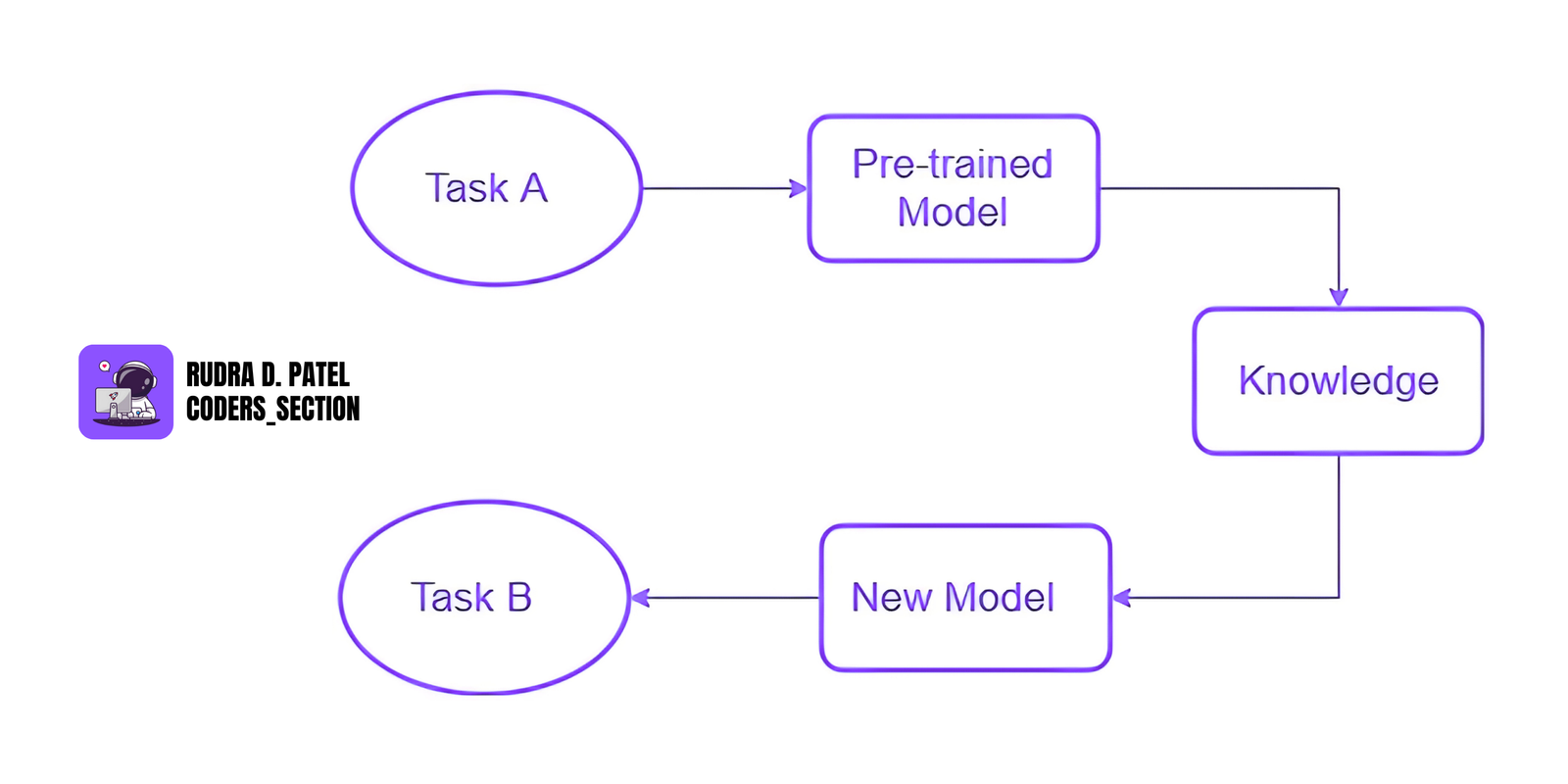
Pre-trained Models

These are models trained on huge datasets.

Examples:

• VGG, ResNet – for images
• BERT – for text

Fine-Tuning

• Slightly updating the pre-trained model using your own smaller dataset.

Feature Extraction

• Using the pre-trained model to extract useful features and then using those features for your own model or task.

Benefit: Saves training time and works well even with limited data.

10.2 Attention Mechanism

This helps the model decide which parts of the input data are most important.

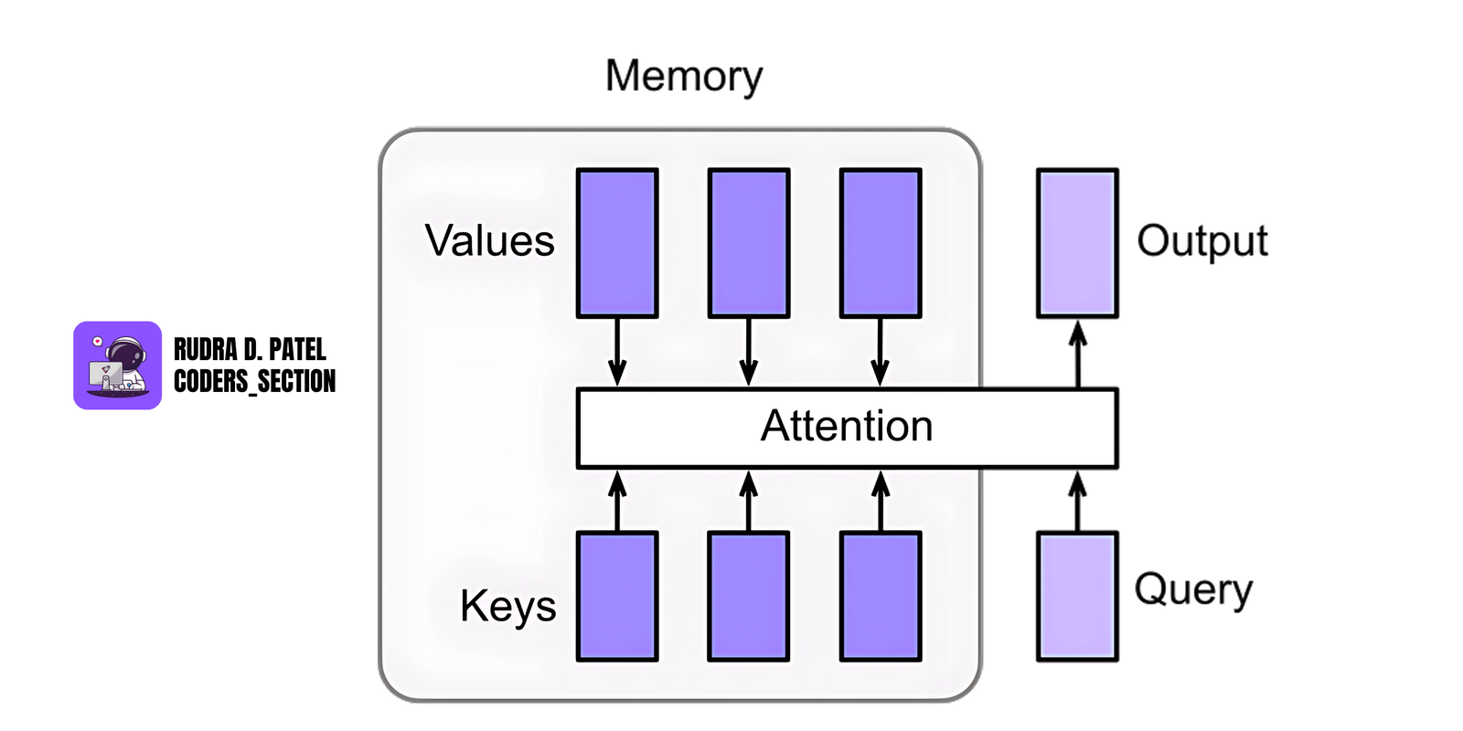
Self-Attention

• Every part of the input focuses on every other part to understand context better.
• Used in NLP (Natural Language Processing) and transformers.

Multi-Head Attention

• Multiple attention mechanisms run in parallel to capture different aspects of relationships in data.

10.3 Reinforcement Learning in Deep Learning

Combining deep learning with reinforcement learning for decision-making tasks.

Actor-Critic

Two models work together:

• Actor: selects the best action
• Critic: evaluates how good the action was

A3C (Asynchronous Advantage Actor-Critic)

• Uses multiple agents to learn in parallel, which speeds up learning and increases stability.

PPO (Proximal Policy Optimization)

• An improved and stable way to train reinforcement learning agents. Used in games, robotics, etc.

10.4 Federated Learning

Model training happens across many devices without collecting data in a central server. Each device keeps its data private and only sends model updates.

Distributed Learning Frameworks

• Used when data is spread across users, hospitals, or devices. Examples include Google’s keyboard predictions.

Privacy-Preserving ML

• Since data never leaves the device, user privacy is protected. This is useful in healthcare, banking, and personal mobile applications.

11.1 Python Libraries

Python is the most popular language in AI/ML. These libraries make your work faster and easier:

• NumPy:
• Used for numerical computing.
• Supports arrays, matrices, and linear algebra operations.
• Pandas:
• Used for data manipulation and analysis.
• You can load data, clean it, and analyze it in tabular formats (DataFrames).
• Scikit-learn:
• A powerful machine learning library.
• Includes ready-to-use models like Linear Regression, SVM, Random Forest, KNN, and more.
• TensorFlow & Keras:
• Used for building deep learning models.
• TensorFlow: low-level control
• Keras: high-level interface, easier to use
• PyTorch:
• An alternative to TensorFlow, widely used in research and development.
• It’s flexible, fast, and dynamic (supports on-the-fly computation graphs).
• OpenCV:
• Used for computer vision tasks like image processing, object detection, face recognition, etc.
• NLTK & SpaCy:
• Libraries for Natural Language Processing (NLP) tasks like tokenization, stemming, sentiment analysis.

11.2 Cloud Platforms

Cloud platforms help you run your models on powerful servers without needing your own hardware.

• Google Colab:
• Free online Jupyter Notebook
• Supports GPU/TPU
• Great for students and beginners
• AWS SageMaker:
• Amazon’s cloud ML platform
• Supports training, tuning, and deploying models at scale
• Used in enterprise-level applications
• Azure ML:
• Microsoft’s machine learning platform
• Integrates well with other Microsoft tools (e.g., Excel, Power BI)
• Provides autoML, drag-and-drop pipelines, and more

12.1 Model Serialization

What it means:

• After training your machine learning model, you save (serialize) it to use later without retraining.

Popular tools:

• Pickle – A Python library to serialize and deserialize Python objects.
• Joblib – Similar to Pickle but better for large NumPy arrays.

Example (Python):

import pickle
from sklearn.linear_model import LogisticRegression

# Train a simple model
model = LogisticRegression()
# model.fit(X_train, y_train) # Assuming X_train, y_train are defined

# Save the model
with open('model.pkl', 'wb') as file:
    pickle.dump(model, file)

# Load the model
with open('model.pkl', 'rb') as file:
    loaded_model = pickle.load(file)
                            

12.2 Flask/Django for Model Deployment

These are web frameworks that let you expose your model as an API endpoint, so other apps or users can access it via the internet.

• Flask: Lightweight and easier for quick ML model APIs.
• Django: Heavier but better for large web applications with built-in admin, security, and ORM.

Flask Example (Python):

from flask import Flask, request, jsonify
import pickle

app = Flask(__name__)

# Load the trained model
with open('model.pkl', 'rb') as file:
    model = pickle.load(file)

@app.route('/predict', methods=['POST'])
def predict():
    data = request.json['data']
    # Assuming 'data' is a list/array that the model can process
    prediction = model.predict([data]).tolist()
    return jsonify({'prediction': prediction})

if __name__ == '__main__':
    app.run(debug=True)
                            

12.3 Serving Models with TensorFlow Serving, FastAPI

TensorFlow Serving:

• Used to deploy TensorFlow models in production. It supports versioning and high-performance serving with REST/gRPC.

FastAPI:

• A modern, fast (high-performance) framework for building APIs with automatic docs, great for production-grade ML APIs.

FastAPI Example (Python):

from fastapi import FastAPI
from pydantic import BaseModel
import pickle

app = FastAPI()

# Load the trained model
with open('model.pkl', 'rb') as file:
    model = pickle.load(file)

class Item(BaseModel):
    data: list[float]

@app.post("/predict/")
async def predict_item(item: Item):
    prediction = model.predict([item.data]).tolist()
    return {"prediction": prediction}
                            

12.4 Monitoring and Maintaining Models in Production

Once your model is live, you need to ensure it continues to perform well.

What to monitor:

• Model accuracy degradation (due to data drift)
• Response time
• Error rates
• System metrics (CPU, memory)

Tools:

• Prometheus + Grafana for system and application monitoring
• MLflow or Evidently.ai for tracking model performance over time

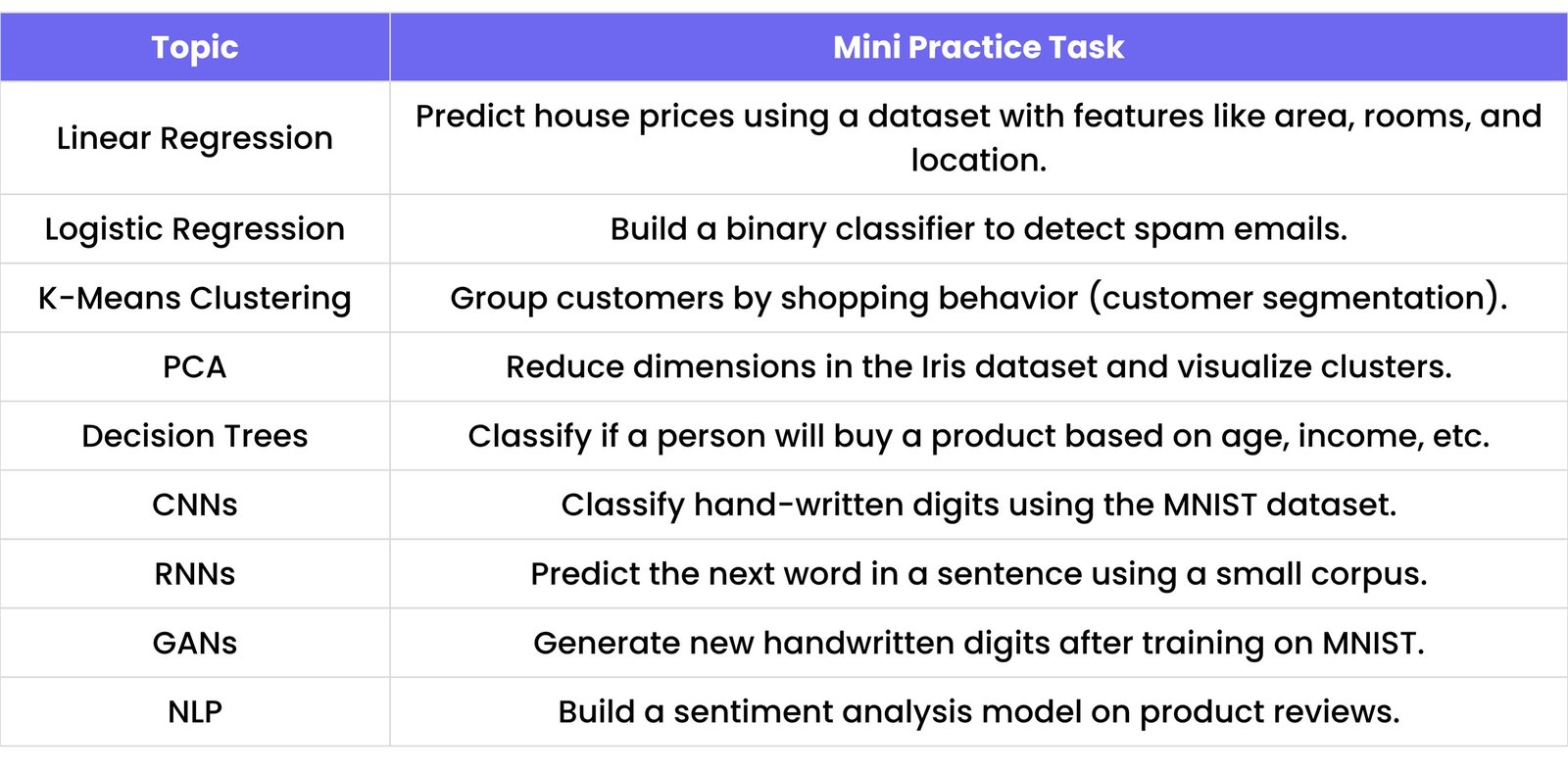
13.1 Practice Tasks

To strengthen understanding, here are simple practice tasks for each core concept:

13.2 Common Beginner Mistakes

General ML Mistakes

• Using test data during training
• Not normalizing/scaling features
• Ignoring class imbalance in classification tasks
• Forgetting to check for data leakage
• Not splitting the data