DSA Cheatsheet

2.1 Prime Numbers

• Prime numbers are numbers greater than 1 that only divide evenly by 1 and themselves.
• Examples: 2, 3, 5, 7, 11.
• Primes are important in encryption and algorithms.
• To check if a number is prime, try dividing it by every number from 2 up to its square root. If any divides evenly, it's not prime.

2.2 GCD and LCM (Euclidean Algorithm)

• GCD (Greatest Common Divisor): The biggest number that divides two numbers without remainder.
• LCM (Least Common Multiple): The smallest number divisible by two numbers.
• Euclidean Algorithm is a fast way to find GCD: Keep dividing the bigger number by the smaller one, replace numbers, until remainder is 0. The last non-zero remainder is the GCD.
• LCM can be found using GCD by formula: $LCM(a, b) = (a \times b) / GCD(a, b)$

2.3 Modular Arithmetic

• Imagine a clock - after 12 hours, it resets to 1.
• Modular arithmetic works the same way, "wrapping around" numbers. Useful to keep numbers small in big calculations (like 1000000007 in coding contests).
• Example: $(8+7) \pmod 5 = 15 \pmod 5 = 0$

2.4 Sieve of Eratosthenes

• A method to find all prime numbers up to a number $n$ quickly.
• How it works:
  • Start with a list of all numbers marked as prime.
  • Start with 2, remove all its multiples.
  • Move to the next number still marked prime and remove its multiples.
  • Continue until you reach the square root of $n$.
  • At the end, the numbers still marked prime are the primes.

2.5 Fast Exponentiation

• If you want to calculate $a^b$ ($a$ to the power $b$), doing $a \times a \times a \dots b$ times takes a long time.
• Fast exponentiation reduces the steps by using:
  • If $b$ is even, $a^b = (a^{b/2}) \times (a^{b/2})$
  • If $b$ is odd, $a^b = a \times (a^{b-1})$
• This method uses divide and conquer to calculate power in $O(\log b)$ steps.

2.6 Bit Manipulation Basics

• Computers work in bits (0s and 1s).
• Bit manipulation means changing or checking individual bits for quick math or logic.
• Important bit operations:
  • AND (&): Both bits 1 $\rightarrow$ 1, else 0
  • OR (|): At least one bit 1 $\rightarrow$ 1
  • XOR (^): Bits different $\rightarrow$ 1, else 0
  • NOT (~): Flip bits (0 $\rightarrow$ 1, 1 $\rightarrow$ 0)
  • Left shift (<<): Multiply by 2
  • Right shift (>>): Divide by 2
• Example: Check if a number is even or odd by num & 1 (1 means odd).

3.1 Introduction to Arrays

• An array is a collection of items stored next to each other in memory.
• You can access each item using its index (starting from 0).
• Example: [10, 20, 30, 40], arr[2] is 30.

3.2 Traversal, Insertion, Deletion

• Traversal: Going through each element one by one.
• Insertion: Adding an element at a position.
• Deletion: Removing an element from a position.
• In arrays, insertion and deletion in the middle need shifting elements, which takes time ($O(n)$).

3.3 Prefix Sum & Sliding Window

• Prefix Sum: Pre-calculated sums from the start up to each position. Helps find sum of any subarray quickly.
• Example: If prefix sums are [2, 5, 9, 14], sum from index 1 to 3 is $14-2 = 12$.
• Sliding Window: Technique to find results over a continuous window of size k. Instead of summing all elements each time, update by removing left element and adding right element.

3.4 Two Pointer Technique

• Use two pointers (indexes) moving through the array.
• Useful for sorted arrays to find pairs or subarrays.
• Move pointers based on condition to reach solution faster.

3.5 Kadane's Algorithm (Max Subarray Sum)

• Find the contiguous subarray with the maximum sum.
• Keep track of current subarray sum and max sum so far.
• If current sum becomes negative, reset it to zero (start a new subarray).

3.6 Sorting Techniques

• Sorting means arranging numbers in order (ascending or descending).
• Some simple sorting methods:
  • Bubble Sort: Compare neighbors, swap if out of order. Repeat.
  • Selection Sort: Find smallest item and place it at the start.
  • Insertion Sort: Build sorted array by inserting one element at a time.
• Faster, advanced sorting methods:
  • Merge Sort: Divide array into halves, sort each half, merge them.
  • Quick Sort: Pick a pivot, partition array around pivot, sort partitions.

4.1 String Basics and Operations

• A string is a sequence of characters, like "hello" or "123abc".
• Strings are stored as arrays of characters.
• Basic operations:
  • Access characters by index (str[0] = 'h')
  • Concatenate strings ("hello" + " world" = "hello world")
  • Length gives number of characters
  • Substring extracts part of a string

4.2 Palindrome Check

• A palindrome reads the same forwards and backwards.
• Example: "madam", "racecar"
• How to check? Compare characters from start and end moving towards center. If all pairs match, it’s a palindrome.

4.3 Anagram Check

• Two strings are anagrams if they have the same letters in any order.
• Example: "listen" and "silent"
• How to check? Sort both strings and compare. Or count character frequency and compare counts.

4.4 String Matching Algorithms

These algorithms find if a pattern exists inside a text.

• Naive algorithm: Check every position in text if pattern matches. Simple but slow for big data ($O(n \times m)$).
• KMP (Knuth-Morris-Pratt): Uses a prefix table to avoid repeating comparisons. Faster.
• Rabin-Karp: Uses hashing to efficiently compare substrings.

4.5 Z-Algorithm

• Calculates an array (Z-array) which tells how many characters from a position match the prefix of the string.
• Helps in pattern searching and string problems.
• Runs in $O(n)$ time.

4.6 Manacher’s Algorithm (Advanced)

• Finds the longest palindromic substring in a string efficiently.
• Runs in $O(n)$ time (much faster than checking all substrings).
• Complex but useful in advanced string problems.

5.1 Singly Linked List

• A linked list is a chain of nodes.
• Each node has data and a pointer to the next node.
• Singly linked list means each node points only to the next node.

5.2 Doubly Linked List

• Each node has a pointer to the next and previous nodes.
• Can move forward and backward easily.

5.3 Circular Linked List

• The last node points back to the head node.
• Can be singly or doubly linked.
• Useful for applications like round-robin scheduling.

5.4 Operations: Insert, Delete, Reverse

• Insert: Add node at beginning, end, or middle.
• Delete: Remove a node by value or position.
• Reverse: Change pointers so list order reverses.

5.5 Detect Cycle (Floyd’s Algorithm)

• Sometimes linked list has a cycle (loop).
• Floyd’s Cycle Detection (Tortoise and Hare): Use two pointers moving at different speeds. If they meet, cycle exists.

5.6 Intersection Point, Merge Two Lists

• Intersection point: Where two linked lists merge. Find by comparing nodes or using difference in lengths.
• Merge two sorted lists: Combine into one sorted list by iterating through both and picking the smaller element.

6.1 Stack Basics

• Stack is a Last In, First Out (LIFO) data structure.
• Imagine a stack of books: the last book you put on top is the first one you take off.

6.2 Push/Pop Operations

• Push: Add element on top of stack.
• Pop: Remove element from top of stack.
• Both operations run in $O(1)$ time.

6.3 Infix to Postfix/Prefix Conversion

• Infix expression: Operators between operands (e.g. A + B).
• Postfix expression: Operators after operands (e.g. A B +).
• Prefix expression: Operators before operands (e.g. + A B).
• Why convert? Easier to evaluate postfix or prefix expressions programmatically.
• How stacks help? Use stack to hold operators and decide order based on precedence.

6.4 Valid Parentheses

• Check if every opening bracket has a matching closing bracket in correct order.
• How to check? Traverse string. Push opening brackets onto stack. When a closing bracket found, pop stack and check if it matches the type.

6.5 Next Greater Element

• For each element in array, find the next element to the right that is greater.
• Can be solved efficiently using a stack.

7.1 Queue Basics

• Definition: A Queue is a linear data structure that follows the First In First Out (FIFO) principle.
• Analogy: Like people standing in a line — the person who enters first gets served first.
• Operations: Enqueue (add element at rear), Dequeue (remove element from front), Peek/Front (see the front element), isEmpty (check if the queue is empty).
• Use Cases: Print queues, task scheduling, real-time systems.

7.2 Circular Queue

• Problem in normal queue: After many dequeues, front moves forward and space at the start is wasted.
• Solution: Circular Queue wraps around and uses space efficiently.
• Circular behavior: When rear reaches the end, it goes to index 0 if space is available.
• Implemented using: Arrays with modular arithmetic:

  
  # For a circular queue of size N
  rear = (rear + 1) % N
  front = (front + 1) % N
                                      

7.3 Deque (Double Ended Queue)

• Definition: A Deque allows insertion and deletion from both front and rear ends.
• Operations: pushFront, pushRear, popFront, popRear.
• Use Cases: Palindrome checker, sliding window problems, browser history.

7.4 Priority Queue / Heap

• Priority Queue: Elements are served based on priority instead of order.
• Implementation: Usually done using a Heap.
• Types: Min-Heap (smallest element at top), Max-Heap (largest element at top).
• Use Cases: CPU scheduling, Dijkstra’s algorithm (shortest path), Top K frequent elements.

7.5 Stack using Queue and vice versa

• Stack using Queue: Use 2 queues. For push, enqueue in one. For pop, dequeue all except last and swap.
• Queue using Stack: Use 2 stacks. For enqueue, push normally. For dequeue, reverse the stack using the second one.

8.1 Recursion Basics

• What is recursion? A function calling itself to solve smaller subproblems.
• Every recursive function has:
  • Base case: Condition to stop recursion.
  • Recursive case: Calls itself with smaller input.

8.2 Factorial, Fibonacci

• Factorial(n): $n! = n \times (n-1)!$

  
  # Python Example: Factorial
  def factorial(n):
      if n == 0 or n == 1: # Base case
          return 1
      return n * factorial(n - 1) # Recursive call
                                      

• Fibonacci(n): $f(n) = f(n-1) + f(n-2)$. Use memoization or DP to avoid recomputation.

8.3 Tower of Hanoi

• Problem: Move $n$ disks from source to destination using helper rod.
• Rules: Move only one disk at a time. Larger disk cannot be placed on a smaller one.
• Recursive logic:
  1. Move $n-1$ disks to helper.
  2. Move $n^{th}$ disk to destination.
  3. Move $n-1$ disks from helper to destination.

8.4 N-Queens Problem

• Goal: Place N queens on N×N board so that no two queens attack each other.
• Approach: Backtracking — try placing a queen in each row and check for safety.
• Key function: isSafe(row, col) checks if it’s safe to place queen at that position.

8.5 Sudoku Solver

• Problem: Fill a 9x9 board so every row, column, and 3x3 box has numbers 1 to 9 without repetition.
• Approach: Backtracking. Try numbers from 1–9 at each empty cell. If valid, move to next cell. If not valid, backtrack.

8.6 Subset / Permutation / Combination Generation

• Subset (Power Set): Include or exclude each element.

# Python Example: Generating Subsets
def subsets(nums, i, current_subset):
    if i == len(nums):
        print(current_subset) # Or add to a result list
        return
    
    # Include current element
    current_subset.append(nums[i])
    subsets(nums, i + 1, current_subset)
    current_subset.pop() # Backtrack

    # Exclude current element
    subsets(nums, i + 1, current_subset)
                                

• Permutations: Swap each element and recurse.
• Combinations: Choose k elements from n without caring about order.

9.1 Linear Search

• Definition: Linear Search is the most basic searching technique. It checks each element of the array one by one until the target element is found or the end is reached.
• Steps: Start from the first element. Compare it with the target. If it matches, return the index. If not, move to the next element. If you reach the end without finding the target, return -1.
• Time Complexity: Best Case: $O(1)$ (if target is at the start), Worst Case: $O(n)$ (if target is at the end or not found).
• Use Case: When the array is unsorted or small in size.

# Python Example for Linear Search
def linear_search(arr, target):
    for i in range(len(arr)):
        if arr[i] == target:
            return i # Found
    return -1 # Not found
                                

9.2 Binary Search

• Definition: Binary Search is an efficient algorithm that works on sorted arrays by repeatedly dividing the search interval in half.
• Steps:
  1. Find the middle index.
  2. If the middle element equals the target, return the index.
  3. If the target is smaller, search in the left half.
  4. If the target is larger, search in the right half.
  5. Repeat the process until the search space is empty.
• Time Complexity: Always: $O(\log n)$.
• Use Case: Only when the array is sorted.

# Python Example for Binary Search
def binary_search(arr, target):
    low = 0
    high = len(arr) - 1

    while low <= high:
        mid = low + (high - low) // 2 # Avoids overflow
        if arr[mid] == target:
            return mid
        elif arr[mid] < target:
            low = mid + 1
        else:
            high = mid - 1
    return -1 # Not found
                                

9.3 Binary Search on Answer

• Definition: Used when you're not searching for a specific value in an array, but trying to optimize or find a boundary/limit (e.g., smallest value that satisfies a condition).
• Typical Use Cases: Minimum number of pages a student can read per day (Book Allocation Problem), Minimum time to complete tasks under certain constraints.
• Steps:
  1. Define the search space (e.g., min and max possible answers).
  2. Apply binary search in that range.
  3. Use a helper function to check if a mid value is a valid solution.
  4. Narrow the search space based on the result.
• Example: Finding the minimum number such that a condition becomes true.

9.4 Search in Rotated Sorted Array

• Definition: This is a modified binary search problem where the array is sorted but rotated at some pivot.
• Example: [6, 7, 8, 1, 2, 3, 4, 5] — a sorted array rotated at index 3.
• Steps:
  1. Use binary search.
  2. Check if the left half or right half is sorted.
  3. Adjust search space based on target and sorted half.
• Time Complexity: $O(\log n)$.

# Python Example for Search in Rotated Sorted Array
def search_rotated_array(arr, target):
    low, high = 0, len(arr) - 1

    while low <= high:
        mid = low + (high - low) // 2
        if arr[mid] == target:
            return mid
        
        # Check if left half is sorted
        if arr[low] <= arr[mid]:
            if arr[low] <= target < arr[mid]:
                high = mid - 1
            else:
                low = mid + 1
        # Right half must be sorted
        else:
            if arr[mid] < target <= arr[high]:
                low = mid + 1
            else:
                high = mid - 1
    return -1
                                

9.5 Lower Bound / Upper Bound

• Lower Bound: The first index where the element is greater than or equal to the target. Useful in sorted arrays. Can be found using binary search.
• Upper Bound: The first index where the element is strictly greater than the target.
• Use Case: Binary search-related problems, frequency count, range queries, etc.

# Python Example (using bisect module)
import bisect

arr = [10, 20, 20, 30, 40]
# lower_bound: first index >= target
print(bisect.bisect_left(arr, 20)) # Output: 1
# upper_bound: first index > target
print(bisect.bisect_right(arr, 20)) # Output: 3
                                

10.1 Bubble Sort

• Idea: Repeatedly swap adjacent elements if they’re in the wrong order.
• Steps: Compare 1st and 2nd $\rightarrow$ swap if needed. Move to next pair. After 1st pass $\rightarrow$ largest element goes to the end. Repeat until array is sorted.
• Time: Best: $O(n)$ (if already sorted), Worst: $O(n^2)$.

# Python Example for Bubble Sort
def bubble_sort(arr):
    n = len(arr)
    for i in range(n - 1):
        for j in range(n - i - 1):
            if arr[j] > arr[j+1]:
                arr[j], arr[j+1] = arr[j+1], arr[j] # Swap
                                

10.2 Selection Sort

• Idea: Select the minimum element and place it at the beginning.
• Steps: Find smallest from unsorted part. Swap it with the first unsorted element. Repeat.
• Time: Always $O(n^2)$.

# Python Example for Selection Sort
def selection_sort(arr):
    n = len(arr)
    for i in range(n - 1):
        min_idx = i
        for j in range(i + 1, n):
            if arr[j] < arr[min_idx]:
                min_idx = j
        arr[i], arr[min_idx] = arr[min_idx], arr[i] # Swap
                                

10.3 Insertion Sort

• Idea: Pick one element and place it in the correct position of the sorted part.
• Steps: Start from 2nd element. Compare it with previous elements. Shift elements and insert at correct spot.
• Time: Best: $O(n)$, Worst: $O(n^2)$.

# Python Example for Insertion Sort
def insertion_sort(arr):
    n = len(arr)
    for i in range(1, n):
        key = arr[i]
        j = i - 1
        while j >= 0 and arr[j] > key:
            arr[j + 1] = arr[j]
            j -= 1
        arr[j + 1] = key
                                

10.4 Merge Sort

• Idea: Divide array into halves, sort each half, then merge them.
• Steps: Divide until single-element arrays. Merge two sorted arrays.
• Time: Always $O(n \log n)$.
• Space: $O(n)$.

# Python Example for Merge Sort
def merge_sort(arr):
    if len(arr) > 1:
        mid = len(arr) // 2
        L = arr[:mid]
        R = arr[mid:]

        merge_sort(L)
        merge_sort(R)

        i = j = k = 0

        while i < len(L) and j < len(R):
            if L[i] < R[j]:
                arr[k] = L[i]
                i += 1
            else:
                arr[k] = R[j]
                j += 1
            k += 1

        while i < len(L):
            arr[k] = L[i]
            i += 1
            k += 1

        while j < len(R):
            arr[k] = R[j]
            j += 1
            k += 1
                                

10.5 Quick Sort

• Idea: Pick a pivot, place elements smaller on left, greater on right $\rightarrow$ recursively sort.
• Time: Best: $O(n \log n)$, Worst: $O(n^2)$ (if badly chosen pivot).

# Python Example for Quick Sort
def quick_sort(arr):
    if len(arr) <= 1:
        return arr
    
    pivot = arr[len(arr) // 2]
    left = [x for x in arr if x < pivot]
    middle = [x for x in arr if x == pivot]
    right = [x for x in arr if x > pivot]
    
    return quick_sort(left) + middle + quick_sort(right)
                                

10.6 Heap Sort

• Idea: Use a heap to extract max/min repeatedly and sort.
• Time: $O(n \log n)$.
• Space: $O(1)$ if using inplace heap.

# Python Example for Heap Sort (Conceptual)
import heapq

def heap_sort(arr):
    heapq.heapify(arr) # Build a min-heap
    sorted_arr = []
    while arr:
        sorted_arr.append(heapq.heappop(arr)) # Extract min repeatedly
    return sorted_arr
                                

10.7 Counting Sort

• Idea: Count occurrences and use that to place elements in sorted order. Only for non-negative integers.
• Time: $O(n + k)$ (k = max element).

# Python Example for Counting Sort
def counting_sort(arr):
    max_val = max(arr)
    counts = [0] * (max_val + 1)
    output = [0] * len(arr)

    for num in arr:
        counts[num] += 1

    for i in range(1, len(counts)):
        counts[i] += counts[i-1]

    for i in range(len(arr) - 1, -1, -1):
        output[counts[arr[i]] - 1] = arr[i]
        counts[arr[i]] -= 1
    
    for i in range(len(arr)):
        arr[i] = output[i]
                                

10.8 Radix Sort

• Idea: Sort numbers digit-by-digit using Counting Sort as a subroutine. Only for integers.
• Time: $O(nk)$ (k = number of digits).

# Python Example for Radix Sort (Conceptual)
def counting_sort_exp(arr, exp):
    n = len(arr)
    output = [0] * n
    counts = [0] * 10 # For digits 0-9

    for i in range(n):
        index = (arr[i] // exp) % 10
        counts[index] += 1

    for i in range(1, 10):
        counts[i] += counts[i - 1]

    i = n - 1
    while i >= 0:
        index = (arr[i] // exp) % 10
        output[counts[index] - 1] = arr[i]
        counts[index] -= 1
        i -= 1
    
    for i in range(n):
        arr[i] = output[i]

def radix_sort(arr):
    max_val = max(arr)
    exp = 1
    while max_val // exp > 0:
        counting_sort_exp(arr, exp)
        exp *= 10
                                

10.9 Bucket Sort

• Idea: Distribute elements into buckets, sort each bucket, then combine.
• Best for uniformly distributed floats (e.g., [0.2, 0.5, 0.8]).
• Time: $O(n + k)$.

# Python Example for Bucket Sort (Conceptual)
def bucket_sort(arr):
    num_buckets = 10 # Example: for values between 0 and 1
    buckets = [[] for _ in range(num_buckets)]

    for num in arr:
        index = int(num * num_buckets)
        buckets[index].append(num)
    
    for i in range(num_buckets):
        buckets[i].sort() # Sort each bucket

    k = 0
    for bucket in buckets:
        for num in bucket:
            arr[k] = num
            k += 1
                                

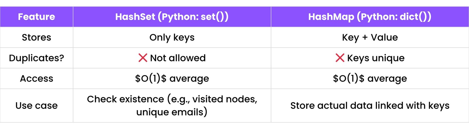
11.1 Hash Table Basics

• A hash table stores key-value pairs.
• Think of it like labeled boxes: You put data inside a box using a key. A hash function turns your key into an index.
• ✅ Fast Access, ❌ Needs good hash function to avoid collisions.

# Python Example: Hash Table (Dictionary)
hash_table = {}
hash_table["apple"] = 1
hash_table["banana"] = 2
print(hash_table["apple"]) # Output: 1
                                

11.2 Frequency Counting

• Used when you want to count how many times something appears (like words, numbers, etc.).
• Example: Count letters in "banana"

  
  # Python Example: Frequency Counting
  s = "banana"
  freq = {}
  for char in s:
      freq[char] = freq.get(char, 0) + 1
  print(freq) # Output: {'b': 1, 'a': 3, 'n': 2}
                                      

• Used in: Finding duplicates, Anagram checking, Word counters.

11.3 HashSet vs HashMap

11.4 Collision Resolution

Sometimes different keys generate the same index. That’s a collision. How to handle it?

• 1. Chaining (Linked Lists in Buckets)
  • Each index holds a list of entries.
  • ✅ Easy to implement, ✅ Saves memory. ❌ Slower if many collisions.

  
  # Python Example: Chaining (Conceptual)
  # hash_table = [[] for _ in range(size)]
  # def insert(key, value):
  #     index = hash_function(key)
  #     hash_table[index].append((key, value))
                                          

• 2. Open Addressing
  • Instead of a list, if a spot is full, find next empty spot.
  • Types: Linear probing (check next cell), Quadratic probing (check $1^2, 2^2, 3^2$ steps away), Double hashing (use second hash).

  
  # Python Example: Open Addressing (Conceptual)
  # hash_table = [None] * size
  # def insert(key, value):
  #     index = hash_function(key)
  #     while hash_table[index] is not None:
  #         index = (index + 1) % size # Linear probing
  #     hash_table[index] = (key, value)
                                          

12.1 Tree Terminology

• Node: Basic unit of a tree containing data.
• Root: The topmost node of the tree.
• Child: A node directly connected to another node when moving away from the root.
• Parent: The node which has children.
• Leaf: A node with no children.
• Subtree: Any node and its descendants.
• Depth: Number of edges from the root to the node.
• Height: Number of edges on the longest path from the node to a leaf.
• Binary Tree: A tree where each node has at most two children (left and right).

12.2 Binary Trees

• A binary tree is a tree where each node has at most two children.
• Example structure: Each node has a left and right pointer.

# Python Node definition for a Binary Tree
class Node:
    def __init__(self, data):
        self.data = data
        self.left = None
        self.right = None
                                

12.3 Binary Search Trees (BST)

• A special kind of binary tree where: Left subtree has values less than the node. Right subtree has values greater than the node.
• This allows fast search, insert, and delete operations in $O(\log n)$ time (if the tree is balanced).

# Python BST Insert Example (Conceptual)
def insert(root, key):
    if root is None:
        return Node(key)
    if key < root.data:
        root.left = insert(root.left, key)
    elif key > root.data:
        root.right = insert(root.right, key)
    return root
                                

12.4 Tree Traversals

• Ways to visit each node in a tree:
  • Inorder (Left, Root, Right): Used in BSTs to get sorted order.
  • Preorder (Root, Left, Right): Used to copy the tree.
  • Postorder (Left, Right, Root): Used to delete the tree.
  • Level-order: Visit level by level (uses queue).
• Example (Inorder):

  
  # Python Inorder Traversal
  def inorder_traversal(root):
      if root is None:
          return
      inorder_traversal(root.left)
      print(root.data, end=" ")
      inorder_traversal(root.right)
                                      

12.5 Height and Diameter of a Tree

• Height: Length of the longest path from root to a leaf.
• Diameter: Longest path between any two nodes (may or may not pass through root).

# Python Height of a Binary Tree
def height(root):
    if root is None:
        return 0
    return 1 + max(height(root.left), height(root.right))

# Python Diameter of a Binary Tree (Conceptual)
# This often requires a pair of (diameter, height) to be returned from recursive calls.
# def diameter_util(root):
#     if root is None:
#         return 0, 0 # diameter, height
#     
#     left_diameter, left_height = diameter_util(root.left)
#     right_diameter, right_height = diameter_util(root.right)
#     
#     current_diameter = left_height + right_height # Path through current root
#     max_diameter = max(current_diameter, left_diameter, right_diameter)
#     current_height = 1 + max(left_height, right_height)
#     
#     return max_diameter, current_height
#
# def diameter(root):
#     d, _ = diameter_util(root)
#     return d
                                

12.6 LCA (Lowest Common Ancestor)

• LCA of two nodes is the deepest node that is an ancestor of both.
• In a Binary Tree:

  
  # Python LCA in a Binary Tree (Conceptual)
  def find_lca(root, n1, n2):
      if root is None or root.data == n1 or root.data == n2:
          return root
      
      left_lca = find_lca(root.left, n1, n2)
      right_lca = find_lca(root.right, n1, n2)
  
      if left_lca and right_lca:
          return root # Found LCA
      elif left_lca:
          return left_lca
      else:
          return right_lca
                                      

12.7 Balanced Binary Tree

• A binary tree is balanced if for every node: Height of left and right subtrees differ by at most 1.

# Python Check if Balanced Binary Tree (Conceptual)
# Returns height if balanced, -1 if unbalanced
def is_balanced_util(root):
    if root is None:
        return 0

    left_height = is_balanced_util(root.left)
    if left_height == -1:
        return -1

    right_height = is_balanced_util(root.right)
    if right_height == -1:
        return -1

    if abs(left_height - right_height) > 1:
        return -1

    return 1 + max(left_height, right_height)

def is_balanced(root):
    return is_balanced_util(root) != -1
                                

12.8 AVL Tree (Advanced)

• AVL Tree is a self-balancing binary search tree. After every insertion or deletion, the tree checks and restores the balance using rotations.
• Properties: Balance factor = height(left) - height(right). Balance factor must be -1, 0, or 1.
• Used where frequent insertions/deletions occur.

12.9 Segment Tree (Advanced)

• Segment Tree is a tree used for storing information about intervals or segments.
• Useful for: Range minimum query, Range sum query, Range updates.
• Construction takes $O(n)$, queries and updates in $O(\log n)$.
• Used in competitive programming and data range queries.

13.1 Trie Basics

• Trie is a tree where each node represents a character of a word.
• The root node is empty, and each path from root to a node spells out a word/prefix.
• Mainly used for autocomplete, prefix searching, and spell checking.
• Example: Words: cat, cap, can. Structure: Each path forms a word starting from the root.

# Python Conceptual Trie Node
class TrieNode:
    def __init__(self):
        self.children = {}
        self.is_end_of_word = False
                                

13.2 Insert & Search Words

• Insert: Start from root. For each character in the word: If node for the character doesn't exist, create it. After last character, mark node as end of word.
• Search: Traverse character by character from root. If path breaks, word not found. If final character reached and node is marked end, word exists.

# Python Trie Insert (Conceptual)
class Trie:
    def __init__(self):
        self.root = TrieNode()

    def insert(self, word: str) -> None:
        curr = self.root
        for char in word:
            if char not in curr.children:
                curr.children[char] = TrieNode()
            curr = curr.children[char]
        curr.is_end_of_word = True

    # Python Trie Search (Conceptual)
    def search(self, word: str) -> bool:
        curr = self.root
        for char in word:
            if char not in curr.children:
                return False
            curr = curr.children[char]
        return curr.is_end_of_word
                                

13.3 Prefix Matching

• Used to check if any word in the Trie starts with a given prefix.
• Same as search, but you don’t check for is_end_of_word. Just ensure all prefix characters exist in the Trie.

# Python Trie StartsWith (Conceptual)
class Trie:
    # ... (init and insert methods)
    def startsWith(self, prefix: str) -> bool:
        curr = self.root
        for char in prefix:
            if char not in curr.children:
                return False
            curr = curr.children[char]
        return True
                                

13.4 Word Suggestions (Autocomplete)

• Given a prefix, return all words in the Trie that begin with it.
• First, find the node for the prefix. Then do a DFS from that node to collect all words.
• Example: If Trie contains ["car", "cat", "cart", "care"]: suggestions("ca") $\rightarrow$ ["car", "cart", "care", "cat"]

# Python Word Suggestions (Conceptual)
class Trie:
    # ... (init, insert, search, startsWith methods)
    def _collect_words(self, node, current_word, results):
        if node.is_end_of_word:
            results.append(current_word)
        for char, child_node in node.children.items():
            self._collect_words(child_node, current_word + char, results)

    def get_suggestions(self, prefix: str) -> list[str]:
        curr = self.root
        for char in prefix:
            if char not in curr.children:
                return [] # No words with this prefix
            curr = curr.children[char]
        
        results = []
        self._collect_words(curr, prefix, results)
        return results
                                

14.1 Graph Representation

• 1. Adjacency List
  • Each node stores a list of its neighbors. Efficient for sparse graphs.
  • Example:

    
    # Python Adjacency List for an undirected graph
    graph = {
        0: [1, 2],
        1: [0, 3],
        2: [0, 3],
        3: [1, 2]
    }
                                                

• 2. Adjacency Matrix
  • A 2D array where matrix[i][j] = 1 if edge exists. Good for dense graphs, but uses more space.
  • Example:

    
    # Adjacency Matrix (Conceptual)
    # For a graph with 3 vertices (0, 1, 2)
    # Edges: (0,1), (0,2)
    # matrix = [
    #     [0, 1, 1],
    #     [1, 0, 0],
    #     [1, 0, 0]
    # ]
                                                

14.2 BFS & DFS

• BFS (Breadth-First Search)
  • Level-by-level traversal. Uses queue. Good for shortest path in unweighted graphs.

  
  # Python BFS (Conceptual)
  from collections import deque
  
  def bfs(graph, start):
      visited = set()
      queue = deque([start])
      visited.add(start)
  
      while queue:
          node = queue.popleft()
          # Process node (e.g., print)
          print(node, end=" ")
  
          for neighbor in graph[node]:
              if neighbor not in visited:
                  visited.add(neighbor)
                  queue.append(neighbor)
                                          

• DFS (Depth-First Search)
  • Goes deep before backtracking. Uses stack (or recursion).

  
  # Python DFS (Conceptual)
  def dfs(graph, node, visited):
      visited.add(node)
      # Process node (e.g., print)
      print(node, end=" ")
  
      for neighbor in graph[node]:
          if neighbor not in visited:
              dfs(graph, neighbor, visited)
                                          

14.3 Detect Cycle

• Undirected Graph: Use DFS and check if a visited node is not the parent.
• Directed Graph: Use DFS with a recursion stack to track nodes in the current path.

14.4 Topological Sort

• Works on Directed Acyclic Graphs (DAG).
• Linear ordering of tasks based on dependencies.
• Use DFS or Kahn’s Algorithm (BFS + in-degree).

14.5 Connected Components

• A connected component is a group of nodes where each node is reachable from any other.
• Use DFS/BFS to count all components.

14.6 Bipartite Graph

• A graph is bipartite if nodes can be colored with 2 colors without adjacent nodes having the same color.
• Check using BFS/DFS with coloring.

14.7 Bridges and Articulation Points

• Bridges: Removing the edge increases components.
• Articulation Points: Removing the node increases components.
• Found using DFS + low time & discovery time.

14.8 Dijkstra’s Algorithm

• Finds shortest path in a weighted graph (no negative weights).
• Uses a min-heap (priority queue).

# Python Dijkstra's Algorithm (Conceptual)
import heapq

def dijkstra(graph, start):
    distances = {node: float('inf') for node in graph}
    distances[start] = 0
    pq = [(0, start)] # (distance, node)

    while pq:
        current_distance, current_node = heapq.heappop(pq)

        if current_distance > distances[current_node]:
            continue

        for neighbor, weight in graph[current_node].items(): # Assuming graph stores neighbors with weights
            distance = current_distance + weight
            if distance < distances[neighbor]:
                distances[neighbor] = distance
                heapq.heappush(pq, (distance, neighbor))
    return distances
                                

14.9 Bellman-Ford Algorithm

• Works with negative weights.
• Slower than Dijkstra.
• Runs $V - 1$ times over all edges ($V$ = vertices).

14.10 Floyd-Warshall Algorithm

• All pairs shortest path.
• Time: $O(V^3)$.
• Dynamic Programming-based.

# Python Floyd-Warshall (Conceptual)
# dist[i][j] = min(dist[i][j], dist[i][k] + dist[k][j])
# INF = float('inf')
# for k in range(V):
#     for i in range(V):
#         for j in range(V):
#             if dist[i][k] != INF and dist[k][j] != INF:
#                 dist[i][j] = min(dist[i][j], dist[i][k] + dist[k][j])
                                

14.11 MST (Minimum Spanning Tree)

• Prim’s Algorithm: Start from one node and expand to nearest unvisited nodes. Uses priority queue.
• Kruskal’s Algorithm: Sort all edges, add smallest one if it doesn’t form a cycle. Uses Union-Find (DSU) to detect cycles.

14.12 Union-Find (Disjoint Set Union)

• A structure to manage connected components efficiently.
• Supports: Find (Get root of a node), Union (Connect two components).
• Uses path compression and union by rank for speed.

# Python Union-Find (Conceptual)
# parent = []
# rank = [] # For union by rank

# def make_set(n):
#     global parent, rank
#     parent = list(range(n + 1))
#     rank = [0] * (n + 1)

# def find_set(v):
#     if v == parent[v]:
#         return v
#     parent[v] = find_set(parent[v]) # Path compression
#     return parent[v]

# def union_sets(a, b):
#     a = find_set(a)
#     b = find_set(b)
#     if a != b:
#         if rank[a] < rank[b]:
#             a, b = b, a # Swap to ensure 'a' is the larger tree
#         parent[b] = a
#         if rank[a] == rank[b]:
#             rank[a] += 1
                                

15.1 Activity Selection Problem

• Goal: Select the maximum number of non-overlapping activities.
• Approach: Sort activities by end time. Always pick the next activity that ends the earliest and doesn’t overlap.

# Python Activity Selection Problem
def activity_selection(activities):
    # activities is a list of tuples: (start_time, end_time)
    activities.sort(key=lambda x: x[1]) # Sort by end time

    count = 1
    last_end_time = activities[0][1]

    for i in range(1, len(activities)):
        if activities[i][0] >= last_end_time:
            count += 1
            last_end_time = activities[i][1]
    return count

# Example usage:
# activities = [(1, 2), (3, 4), (0, 6), (5, 7), (8, 9), (5, 9)]
# print("Max activities:", activity_selection(activities)) # Output: 4
                                

15.2 Fractional Knapsack

• Goal: Maximize profit by taking items with given weight and value, but you can take fractions of items.
• Approach: Calculate value/weight ratio for all items. Sort by highest ratio. Take as much as you can from highest ratio item until the bag is full.

# Python Fractional Knapsack
def fractional_knapsack(capacity, items):
    # items is a list of tuples: (value, weight)
    # Sort items by value/weight ratio in descending order
    items.sort(key=lambda x: x[0] / x[1], reverse=True)

    total_value = 0.0
    current_weight = 0

    for value, weight in items:
        if current_weight + weight <= capacity:
            current_weight += weight
            total_value += value
        else:
            remaining_capacity = capacity - current_weight
            total_value += (value / weight) * remaining_capacity
            break # Knapsack is full
    return total_value

# Example usage:
# items = [(60, 10), (100, 20), (120, 30)]
# capacity = 50
# print("Max value:", fractional_knapsack(capacity, items)) # Output: 240.0
                                

15.3 Huffman Encoding

• Goal: Compress data by assigning shorter binary codes to more frequent characters.
• Approach: Build a min heap of characters based on frequency. Merge two smallest nodes until one remains (build tree). Assign binary codes by traversing the tree.
• Used in file compression like .zip, .rar.

15.4 Job Scheduling Problem

• Goal: Maximize profit by doing jobs with deadlines and profits (only one job at a time).
• Approach: Sort jobs by profit (descending). For each job, try to schedule it as late as possible before its deadline.

# Python Job Scheduling (Conceptual)
# jobs = [(profit, deadline), ...]
# jobs.sort(key=lambda x: x[0], reverse=True) # Sort by profit
#
# max_deadline = max(job[1] for job in jobs)
# slots = [False] * (max_deadline + 1) # Track available slots
# total_profit = 0
#
# for profit, deadline in jobs:
#     for i in range(min(deadline, max_deadline), 0, -1):
#         if not slots[i]:
#             slots[i] = True
#             total_profit += profit
#             break
# print("Max profit:", total_profit)
                                

15.5 Coin Change (Greedy)

• Goal: Give change using the minimum number of coins.
• Approach (Greedy): Sort coins in descending order. Pick largest coin possible each time until the amount becomes zero.
• Works when coins are canonical (like Indian coins).
• Note: Greedy may not work for all coin sets (like [9, 6, 1]), where dynamic programming is better.

16.1 Memoization vs Tabulation

• Memoization (Top-Down): Use recursion and store answers to subproblems in a map or array.
• Tabulation (Bottom-Up): Use loops to build up the solution from base cases.

16.2 0/1 Knapsack

• Given weights and values of items, find the maximum value you can get in a bag with limited capacity. Each item can be picked at most once.

16.3 Longest Common Subsequence (LCS)

• Find the longest subsequence (not substring) present in both strings in the same order.

16.4 Longest Increasing Subsequence (LIS)

• Find the length of the longest increasing subsequence in an array.

16.5 Matrix Chain Multiplication

• Given matrices, find the best order to multiply them with the least cost (number of multiplications).

16.6 DP on Subsets, Strings, Grids, Trees

• Subsets: Use bitmasks or recursion + DP for problems like subset sum.
• Strings: Problems like LCS, edit distance use DP.
• Grids: Use 2D DP for path finding, max sum, etc.
• Trees: Use post-order DP for problems like diameter or counting.

16.7 Optimal BST, Egg Dropping, Rod Cutting

• Optimal BST: Minimize search cost using frequency-based DP.
• Egg Dropping: Minimize attempts to find threshold floor using DP.
• Rod Cutting: Maximize profit by cutting rods into pieces.

17.1 Maximum Sum Subarray of Size K

• Find max sum of any subarray of size K.

17.2 Longest Substring Without Repeating Characters

• Find longest substring without duplicate characters.

17.3 Count Anagrams

• Count how many substrings are anagrams of a given pattern.

17.4 Variable Window Size Problems

• Use when window size is not fixed. Example: Smallest window with a given sum.

18.1 AND, OR, XOR, NOT

• Bitwise operations work on bits (0 and 1) of numbers.
• AND (&): 1 only if both bits are 1.
• OR (|): 1 if any bit is 1.
• XOR (^): 1 if bits are different.
• NOT (~): Flips bits (0 $\rightarrow$ 1, 1 $\rightarrow$ 0).

18.2 Checking Even/Odd

• Check last bit using AND with 1. If (n & 1) == 0 $\rightarrow$ even, else odd.

18.3 Set/Clear/Toggle Bits

• Set bit: Turn a bit ON $\rightarrow$ Use OR with (1 << pos).
• Clear bit: Turn a bit OFF $\rightarrow$ Use AND with ~(1 << pos).
• Toggle bit: Flip bit $\rightarrow$ Use XOR with (1 << pos).

18.4 Counting Set Bits

• Count how many 1s are in binary representation.
• Simple way: Check each bit or use n & (n-1) trick to remove last set bit.

18.5 Power of Two Check

• A number is power of two if it has only 1 set bit.
• Check using n & (n-1) == 0 (and n > 0).

18.6 XOR Tricks (Single Number, Two Repeating Numbers)

• XOR of a number with itself is 0.
• XOR all numbers; result is the single number which appears once.
• For two numbers appearing once, use XOR and bit masking to separate.

19.1 Min Heap / Max Heap Basics

• Heap is a complete binary tree with special order:
• Min heap: Parent $\le$ children.
• Max heap: Parent $\ge$ children.
• Supports efficient insertion, deletion of min/max.

19.2 Heapify

• Process to build heap from unordered array.
• Heapify ensures heap property starting from bottom nodes.

19.3 K Largest/Smallest Elements

• Use heap of size K to keep track.
• For largest: use min heap of size K.
• For smallest: use max heap of size K (or invert values).

19.4 Merge K Sorted Lists

• Use a min heap to merge K sorted lists efficiently.
• Push first elements of each list into heap.
• Extract min and push next element from same list until done.

19.5 Median in Stream

• Maintain two heaps: max heap for lower half, min heap for upper half.
• Balancing heaps allows $O(\log n)$ median finding after each insertion.

20.1 Range Sum/Min/Max Queries – Why Do We Need These?

• Let’s say you have an array like this: arr = [2, 4, 5, 7, 8, 9, 1]
• Now imagine you're asked repeatedly: What’s the sum from index 2 to 5? What’s the minimum value between index 0 and 3?
• You can solve this using a for loop in $O(n)$ time for each query. But if you get thousands of queries, it becomes slow.
• That’s where Segment Tree and BIT (Fenwick Tree) help. They allow: Fast range queries (sum, min, max): in $O(\log n)$ time. Fast updates to the array: in $O(\log n)$ time.

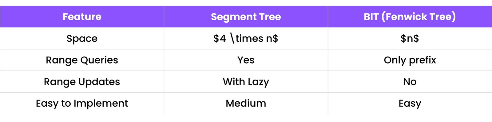
20.2 Segment Tree

• A Segment Tree is a binary tree built on top of an array.
• Each node represents a range of values and stores a result (like sum, min, max) for that range.
• Example: Array: [1, 3, 5, 7]. Segment tree will store: Root = sum(0 to 3) = 16. Left child = sum(0 to 1) = 4. Right child = sum(2 to 3) = 12. And so on...
• Operations: Build Tree: $O(n)$, Range Query (sum/min/max): $O(\log n)$, Update an element: $O(\log n)$.
• Use Case: Imagine a leaderboard of scores – if a score changes or we want to know the sum of top scores.

20.3 Fenwick Tree (Binary Indexed Tree - BIT)

• A Fenwick Tree is another tree-like structure for prefix sums.
• It’s smaller and easier than a Segment Tree but only works with: Point updates (single element), Prefix queries (sum from 1 to i).
• Example Use: Count how many numbers are $\le$ 5 in a dynamic array.
• Operations: Update(index, value) – $O(\log n)$, Query(index) – prefix sum up to index – $O(\log n)$.
• Comparison:

21.1 Union by Rank

• When merging two sets, we attach the smaller tree under the bigger one.
• This keeps the resulting tree short. And short trees mean faster future operations.

21.2 Path Compression

• When you find the "leader" (also called root or parent) of a set, you can flatten the path.
• Let all the children point directly to the root. This makes future searches faster.
• Combined with Union by Rank, this gives almost $O(1)$ time per operation.

21.3 Applications in Graphs (Kruskal's Algorithm)

• In Kruskal’s Algorithm (for Minimum Spanning Tree): You want to add edges without creating cycles. So, before adding an edge between u and v, use DSU: If u and v are in the same set $\Rightarrow$ adding the edge creates a cycle.

22.1 Rabin-Karp Algorithm – Pattern Matching with Hashing

• Use Case: Find all occurrences of a pattern in a long string. Example: Find how many times "abc" appears in "ababcabcabc".
• How It Works: Compute a hash for the pattern (e.g., "abc"). Slide a window of the same size over the main text. For each window, compute its hash and compare with the pattern’s hash. If hash matches $\rightarrow$ double-check by comparing characters.
• Why It's Fast: Hashing allows skipping many unnecessary character-by-character checks. It works in $O(n + m)$ time on average ($n$ = text length, $m$ = pattern length).

22.2 Tarjan’s Algorithm – Strongly Connected Components (SCC)

• Use Case: In a directed graph, find groups of nodes where every node can reach every other in the group. Example: If A $\rightarrow$ B $\rightarrow$ C $\rightarrow$ A, then {A, B, C} is a Strongly Connected Component.
• Why Use It: Useful in circuit design, network analysis, etc.

22.3 Convex Hull – Geometry Problem

• Use Case: Given a set of points on a plane, find the smallest polygon (boundary) that encloses all points. Example: If you have 10 scattered dots on a paper, the convex hull is the rubber band stretched around them.
• Why It’s Important: Used in computer graphics, GIS mapping, collision detection, robotics.
• Popular Algorithms: Graham Scan ($O(n \log n)$), Jarvis March ($O(nh)$, where h = number of hull points).

22.4 MO’s Algorithm – Offline Range Queries

• Use Case: Given multiple queries of form: “What is the frequency of elements between index L to R?” Problem: Doing each query individually is slow for large data.
• MO’s Trick: Sort the queries cleverly using $\sqrt{n}$ blocks (square root decomposition). Process them in that sorted order to minimize data movement. Great for range frequency problems, prefix sums, etc.
• Time Complexity: $O((n + q) \times \sqrt{n})$

22.5 Square Root Decomposition (Sqrt Decomposition)

• Use Case: To handle range queries and point updates faster than brute-force but simpler than Segment Trees.

Final Advice:

• Mistake: Forgetting edge cases $\rightarrow$ Fix: Write test cases manually.
• Mistake: Wrong complexity $\rightarrow$ Fix: Estimate time for large inputs.
• Mistake: Wrong data structure $\rightarrow$ Fix: Understand use-cases.
• Mistake: Recursion bugs $\rightarrow$ Fix: Add base case first.
• Mistake: Off-by-one $\rightarrow$ Fix: Use print/debug to check loop.
• Mistake: Indexing error $\rightarrow$ Fix: Draw array and test logic.
• Mistake: Duplicate issues $\rightarrow$ Fix: Sort input + check previous value.

23.1 Sliding Window Template

• Use Case: Used when dealing with contiguous subarrays or substrings, especially for problems like: Max/min sum of subarray, Longest substring without repeating characters, Count of substrings with some condition.
• Two Types: Fixed Window Size (e.g., size k), Variable Window Size (e.g., until a condition is met).
• Template (Variable Window):

  
  # Python Sliding Window Template (Conceptual)
  # def sliding_window(arr):
  #     left = 0
  #     right = 0
  #     window_sum = 0 # Or other metric
  #     max_length = 0 # Or other result variable
  #     n = len(arr)
  #
  #     while right < n:
  #         # Expand window: Add element at 'right' to window_sum/metrics
  #         window_sum += arr[right]
  #
  #         # Shrink window: Adjust 'left' if condition is not met
  #         while condition_not_met(window_sum, ...): # Define your condition
  #             window_sum -= arr[left]
  #             left += 1
  #
  #         # Update result (e.g., max length, count) after window is valid
  #         max_length = max(max_length, right - left + 1)
  #
  #         right += 1
  #     return max_length
                                      

23.2 Recursion + Memoization Template

• Use Case: Problems that have overlapping subproblems, especially in Dynamic Programming, like: Fibonacci, 0/1 Knapsack, LCS (Longest Common Subsequence).
• Template (Top-down DP):

  
  # Python Recursion + Memoization Template (Conceptual)
  # memo = {} # Dictionary for memoization
  
  # def solve(state):
  #     if state in memo:
  #         return memo[state]
  #
  #     if base_case(state): # Define your base case
  #         return base_value
  #
  #     # Recursive calls to smaller subproblems
  #     result = calculate_recursive_solution(solve(smaller_state_1), solve(smaller_state_2))
  #
  #     memo[state] = result # Store result
  #     return result
                                      

23.3 BFS / DFS Template

• DFS Template (Recursive):
  • Used for: Tree traversals, Connected components, Cycle detection.

  
  # Python DFS Template (Conceptual)
  # def dfs(node, graph, visited):
  #     visited.add(node)
  #     # Process node
  #     for neighbor in graph[node]:
  #         if neighbor not in visited:
  #             dfs(neighbor, graph, visited)
                                          

• BFS Template (Level Order):
  • Used for: Shortest path in unweighted graphs, Level order traversal in trees.

  
  # Python BFS Template (Conceptual)
  # from collections import deque
  #
  # def bfs(start_node, graph):
  #     queue = deque([start_node])
  #     visited = {start_node}
  #
  #     while queue:
  #         curr_node = queue.popleft()
  #         # Process curr_node
  #         for neighbor in graph[curr_node]:
  #             if neighbor not in visited:
  #                 visited.add(neighbor)
  #                 queue.append(neighbor)
                                          

23.4 Binary Search on Answer Template

• Use Case: When the answer lies within a range and the problem asks for min/max valid value.
• Common Examples: Minimum largest subarray sum, Capacity to ship packages in D days, Koko eating bananas (Leetcode).
• Key Idea: Use binary search when: You can define a range (e.g., capacity, time, size), You have a function to check if a guess is valid (is_valid).

# Python Binary Search on Answer Template (Conceptual)
# def is_valid(guess, *args):
#     # Logic to check if 'guess' is a valid solution
#     # Returns True or False
#     pass
#
# def binary_search_on_answer(min_ans, max_ans, *args):
#     low = min_ans
#     high = max_ans
#     ans = max_ans # Initialize with a default or max possible
#
#     while low <= high:
#         mid = low + (high - low) // 2
#         if is_valid(mid, *args):
#             ans = mid
#             high = mid - 1 # Try for a smaller valid answer
#         else:
#             low = mid + 1 # Need a larger answer
#     return ans
                                

24.1 Forgetting to Check Edge Cases

• Example mistakes: Empty array or string, Array with only 1 element, Very large/small input values, Duplicates or negative numbers.
• Tip: Always ask: "What happens if the input is empty or at its limits?"

24.2 Not Understanding Time and Space Complexity

• Mistake: Writing a solution that is correct but too slow.
• Why it matters: If your code runs in $O(n^2)$ on large inputs (like $n = 10^5$), it may timeout or crash.
• Tip: Analyze each loop and recursion to estimate complexity.

24.3 Using the Wrong Data Structure

• Example: Using a list to search elements ($O(n)$) instead of a set ($O(1)$). Using arrays instead of heaps for priority queues.
• Tip: Learn which data structure fits which problem:
  • Set for lookup
  • Queue/Stack for order
  • Heap for top-k
  • HashMap for counting

24.4 Confusing Recursion Base Case

• Mistake: Forgetting the base case or defining it incorrectly, leading to infinite recursion or incorrect results.
• Tip: Always define the simplest possible input for which the answer is known directly.

24.5 Ignoring Input Constraints

• Mistake: Using brute force when $n$ is very large.
• Tip: Read constraints carefully: If $n \le 10^5$, use $O(n \log n)$. If $n \le 20$, brute force may be fine.

24.6 Off-by-One Errors in Loops

• Mistake: Using <= instead of < in loops or starting at the wrong index.
• Tip: Draw small input examples and trace the loop.

24.7 Mistakes in Indexing Arrays or Strings

• Common Errors: Going out of bounds, Using wrong start/end in slicing.
• Tip: Use debugging prints or assert statements.

24.8 Not Handling Duplicates Properly

• Example Mistake: Counting or skipping duplicates wrongly in problems like: Two Sum, Subsets, Combinations.
• Tip: Sort the input if needed and add logic to skip duplicates.

Final Advice:

• Mistake: Forgetting edge cases $\rightarrow$ Fix: Write test cases manually.
• Mistake: Wrong complexity $\rightarrow$ Fix: Estimate time for large inputs.
• Mistake: Wrong data structure $\rightarrow$ Fix: Understand use-cases.
• Mistake: Recursion bugs $\rightarrow$ Fix: Add base case first.
• Mistake: Off-by-one $\rightarrow$ Fix: Use print/debug to check loop.
• Mistake: Indexing error $\rightarrow$ Fix: Draw array and test logic.
• Mistake: Duplicate issues $\rightarrow$ Fix: Sort input + check previous value.