Data Analysis Cheatsheet

2.1 Descriptive Statistics

• Descriptive statistics summarize and describe the key features of a dataset. This is usually the first step to understand the data before any advanced analysis.

2.1.1 Mean, Median, Mode

Mean (Average):

• The mean is calculated by adding all values and then dividing by the number of values. It represents the "central" value of the dataset.

Example: For the data $[3, 5, 7]$, mean $=(3+5+7)/3=5$

Median (Middle Value):

• The median is the middle number when data points are arranged in order. If there is an even number of points, the median is the average of the two middle values. The median is less affected by extreme values (outliers) than the mean.

Example: For $[1, 3, 7]$, median is 3. For $[1, 3, 7, 9]$, median is $(3+7)/2=5$.

Mode (Most Frequent):

• The mode is the value that appears most frequently in the dataset. A dataset may have more than one mode or no mode at all if all values are unique.

Example: In $[2, 4, 4, 6, 7]$, mode is 4.

2.1.2 Variance and Standard Deviation

Variance:

• Variance measures how far each data point is from the mean, on average. It is the average of squared differences between each value and the mean. Larger variance means data points are more spread out.

Formula:

$Variance=\frac{1}{N}\sum_{i=1}^{N}(x_{i}-\mu)^{2}$

• Where $x_i$ are the data points and $\mu$ is the mean.

Standard Deviation (SD):

• The standard deviation is the square root of the variance. It is easier to interpret because it is in the same units as the data. A small SD means data points cluster near the mean; a large SD means they are more spread out.

2.1.3 Quartiles, Range, and Interquartile Range (IQR)

Range:

• The simplest measure of spread: maximum value minus minimum value.

Example: For $[2, 5, 9]$, range $=9-2=7$

Quartiles:

• Quartiles divide data into four equal parts.
• Q1 (First quartile): 25th percentile
• Q2 (Second quartile or median): 50th percentile
• Q3 (Third quartile): 75th percentile

Interquartile Range (IQR):

• IQR is the range of the middle 50% of data and is calculated as
• $IQR=Q3-Q1$
• It's a robust measure of variability, less sensitive to outliers.

2.2 Probability Basics

• Probability quantifies how likely an event is to happen, expressed between 0 (impossible) and 1 (certain).

2.2.1 Basic Probability Rules

• Probability of an event A:

$P(A)=$ Number of favorable outcomes / Total number of outcomes

• The sum of probabilities of all possible outcomes equals 1.
• Complement Rule:
• Probability that event A does not happen is:

$P(A^{c})=1-P(A)$

2.2.2 Conditional Probability

• Conditional probability measures the probability of event A occurring given that event B has occurred:

$P(A|B) = P(A \cap B) / P(B)$

• This is useful when events are dependent on each other.

2.2.3 Bayes' Theorem

• Bayes' theorem allows us to update the probability of an event based on new information:

$P(A|B) = (P(B|A) \times P(A)) / P(B)$

• It's widely used in medical testing, spam filtering, and machine learning.

2.2.4 Probability Distributions

Normal Distribution:

• Known as the bell curve, symmetric around the mean, many natural phenomena follow this pattern.

Binomial Distribution:

• Models the number of successes in fixed number of independent yes/no experiments (trials), with constant success probability.

Poisson Distribution:

• Describes the number of times an event occurs in a fixed interval of time or space when events happen independently and at a constant average rate.

2.3 Inferential Statistics

• Inferential statistics allow us to make conclusions about a large population based on a smaller sample.

2.3.1 Hypothesis Testing

Null Hypothesis (H₀):

• A statement that there is no effect or difference.

Alternative Hypothesis (H₁):

• A statement that there is an effect or difference.

2.3.2 P-Value and Confidence Intervals

P-Value:

• The probability of obtaining the observed results if the null hypothesis were true.
• If the p-value is less than a predetermined significance level (commonly 0.05), we reject the null hypothesis.

Confidence Interval (CI):

• A range of values within which we expect the true population parameter to lie, with a certain confidence level (e.g., 95%).

2.3.3 Z-Test and T-Test

Z-Test:

• Used when the sample size is large (usually >30) and population variance is known.

T-Test:

• Used when the sample size is small and population variance is unknown.

Both tests compare means to check if there is a statistically significant difference between groups.

2.3.4 Chi-Square Test

• Used to determine if there is a significant association between two categorical variables.

Example: Testing if gender and preferred product type are related.

2.3.5 ANOVA (Analysis of Variance)

• Used when comparing means across three or more groups to see if at least one group mean is different from the others.

2.4 Correlation and Covariance

• These measure how two variables change together.

2.4.1 Pearson and Spearman Correlation Coefficients

Pearson Correlation:

• Measures the strength and direction of a linear relationship between two continuous variables.
• Values range from -1 to +1.

Spearman Correlation:

• A non-parametric measure that assesses how well the relationship between two variables can be described by a monotonic function (used for ranked data).

2.4.2 Covariance Matrix

• A matrix showing covariances between multiple variables. It indicates how variables vary together. Positive values mean variables increase together, negative means one increases while the other decreases.

2.4.3 Correlation vs. Causation

• Correlation means two variables change together but does not imply one causes the other.
• Causation means one variable directly affects the other.

Data collection is the first and most crucial step in the data analysis process. It involves gathering data from various sources in different formats. This section explains the types of data, where it comes from, and how it can be collected.

3.1 Types of Data

Understanding the type of data you're dealing with helps in choosing the right analysis method and tools.

3.1.1 Structured vs. Unstructured Data

Structured Data:

• Data that is organized in a defined format such as rows and columns. It is easy to store in databases and analyze using standard tools.

Examples: Excel sheets, SQL databases, sales records.

Unstructured Data:

• Data that does not follow a fixed format. It’s often more complex and harder to analyze.

Examples: Text, images, videos, social media posts, emails.

3.1.2 Qualitative vs. Quantitative Data

Qualitative Data:

• Describes qualities or characteristics. It is non-numerical and usually collected through interviews or open-ended surveys.

Examples: Customer reviews, interview transcripts, color.

Quantitative Data:

• Numerical data that can be measured or counted.

Examples: Age, income, sales figures.

3.2 Data Sources

Data can come from various sources:

3.2.1 Databases (SQL, NoSQL)

• SQL Databases (Relational): Store structured data in tables (e.g., MySQL, PostgreSQL, SQL Server).
• NoSQL Databases (Non-relational): Store unstructured or semi-structured data (e.g., MongoDB, Cassandra).

3.2.2 CSV, Excel, JSON, APIs

• CSV (Comma Separated Values): Simple text files for tabular data.
• Excel: Spreadsheets for organizing and analyzing data.
• JSON (JavaScript Object Notation): Lightweight data-interchange format, often used in web APIs.
• APIs (Application Programming Interfaces): Allow programs to communicate and exchange data.

3.2.3 Web Scraping

• The process of extracting data from websites using tools or scripts.
• Used when data is not available through APIs. Requires careful handling to comply with website terms and conditions.

Tools: Python (BeautifulSoup, Scrapy), Selenium.

3.3 Data Acquisition Methods

There are different ways to gather data depending on the purpose and context.

3.3.1 Surveys and Questionnaires

• Used to collect opinions, feedback, and preferences directly from people.
• Can be conducted online (Google Forms, Typeform) or offline.
• Effective for collecting qualitative and quantitative data.

3.3.2 Sensor Data and IoT Devices

• Devices like temperature sensors, fitness trackers, and smart home appliances generate continuous data.
• Common in real-time monitoring, environmental data, health tracking, etc.

3.3.3 Public Datasets

• Pre-collected datasets made available for public use in learning and research.

Examples:

• Kaggle: Offers datasets for machine learning and data science competitions.
• UCI Machine Learning Repository.

Before analyzing data, we must clean and prepare it. Raw data usually contains errors, missing values, and inconsistencies. Preprocessing ensures the data is accurate and ready for analysis.

4.1 Handling Missing Data

Missing values are common in real-world datasets and must be treated carefully to avoid misleading results.

4.1.1 Imputation (Mean, Median, Mode)

• Mean Imputation: Replace missing values with the average of that column.
• Median Imputation: Use the middle value; best for skewed data.
• Mode Imputation: Use the most frequent value; ideal for categorical data.

4.1.2 Dropping Missing Data

• Remove rows or columns with missing values.
• Used only when missing data is minimal and won't affect results.

4.1.3 Forward/Backward Filling

• Forward Fill: Replace missing value with the previous value.
• Backward Fill: Replace missing value with the next available value.
• Useful in time-series data.

4.2 Data Transformation

Changing data into the right format or scale to make it suitable for analysis or modeling.

4.2.1 Scaling and Normalization

• Scaling (Min-Max Scaling): Rescales data to a fixed range (e.g., 0 to 1).
• Normalization (Z-score normalization): Transforms data to have a mean of 0 and standard deviation of 1.

Formula for Z-score:

$Z = (X - \mu) / \sigma$

Where $X$ is the data point, $\mu$ is the mean, and $\sigma$ is the standard deviation.

4.2.2 Encoding Categorical Data (One-Hot Encoding, Label Encoding)

• One-Hot Encoding: Converts categorical data into numerical format by creating new binary columns for each category.
• Label Encoding: Assigns a unique numerical label to each category.

4.3 Handling Outliers

Outliers are data points that are significantly different from other observations. They can skew results and need careful treatment.

4.3.1 Identifying Outliers (Z-Score, IQR)

• Z-Score Method: Data points with Z > 3 or Z < -3 are often considered outliers.
• IQR Method: Outliers lie below $Q1 - 1.5 \times IQR$ or above $Q3 + 1.5 \times IQR$.

4.3.2 Treatment of Outliers

• Capping: Replace extreme values with a boundary value.
• Removal: Delete rows with extreme outliers if they affect the results.

4.4 Data Aggregation and Grouping

Combining data to extract insights based on categories or time frames.

4.4.1 GroupBy Operations

• Used to group data by one or more columns and apply aggregation functions like `sum()`, `mean()`, `count()`.

Example in Python (Pandas):

df.groupby('Category')['Sales'].sum()
                            

4.4.2 Pivot Tables and Cross-Tabulations

• Pivot Table: Summarizes data in a table format using multiple dimensions (like Excel).
• Cross-Tabulation: Shows frequency distribution between two or more categorical variables.

4.5 Data Consistency

Ensuring the data is uniform and duplicates are removed.

4.5.1 Removing Duplicates

• Duplicates can bias analysis and must be identified and removed.

Example in Pandas:

df.drop_duplicates(inplace=True)
                            

4.5.2 Standardizing Data Formats

• Convert all dates, phone numbers, text cases, currency values, etc., to a consistent format.

Example: 01/01/2024 → 2024-01-01 for all date entries.

EDA is the process of visually and statistically examining datasets to understand their structure, patterns, and anomalies before applying any machine learning models. It’s a critical step for data-driven decisions.

5.1 Data Visualization

Visualizations help us understand trends, patterns, and outliers in the data.

5.1.1 Basic Plots

• Histograms: Show the frequency of values in bins. Useful for understanding data distribution.
• Boxplots: Show median, quartiles, and outliers.
• Scatterplots: Display relationships between two numerical variables.

5.1.2 Correlation Heatmaps

• A correlation matrix shows how strongly variables relate to each other (from -1 to 1).
• Heatmaps use colors to show this correlation visually.

Example in Python (Seaborn):

import seaborn as sns
sns.heatmap(df.corr(), annot=True, cmap='coolwarm')
                            

5.1.3 Pairplots, Violin Plots, Bar Plots

• Pairplot: Plots scatterplots for all variable combinations.
• Violin Plot: Combines boxplot and density plot; shows distribution and probability.
• Bar Plot: Used to compare categorical data using heights.

5.1.4 Line Graphs and Area Plots

• Line Graphs: Show trends over time.
• Area Plots: Similar to line graphs but the area between the line and the axis is filled.

5.2 Summary Statistics

• Descriptive Measures (Mean, Median, Mode): As discussed in Section 2.1.1.
• Distribution Analysis (Skewness, Kurtosis):
• Skewness: Measures the asymmetry of the probability distribution.
• Kurtosis: Measures the "tailedness" of the probability distribution.

5.3 Outlier Detection

5.3.1 Visualizing Outliers

• Boxplots: Points outside whiskers are outliers.
• Scatterplots: Easily show data points that lie far from the rest.

5.3.2 Statistical Tests for Outliers

• Z-Score Method: Data points with Z > 3 or Z < -3 are often considered outliers.
• IQR Method: Outliers lie below $Q1 - 1.5 \times IQR$ or above $Q3 + 1.5 \times IQR$.

5.4 Dimensionality Reduction

Used when datasets have many features (columns), which can be hard to visualize or analyze.

5.4.1 Principal Component Analysis (PCA)

• PCA reduces the number of features while keeping the most important patterns.
• It transforms features into new components that explain maximum variance.

5.4.2 t-SNE (t-Distributed Stochastic Neighbor Embedding)

• A technique to visualize high-dimensional data in 2D or 3D.
• Captures non-linear patterns and clusters better than PCA.
• Commonly used for visualizing clusters in classification problems.

Statistical analysis helps make decisions using data. It includes testing assumptions, measuring relationships, and predicting outcomes.

6.1 Hypothesis Testing

Hypothesis testing is a method to make decisions based on data.

6.1.1 Null and Alternative Hypothesis

• Null Hypothesis (H₀): A statement that there is no effect or difference. Example: "There is no difference in test scores between two groups."
• Alternative Hypothesis (H₁): A statement that there is an effect or difference.

6.1.2 Type I and Type II Errors

• Type I Error (False Positive): Rejecting the null hypothesis when it is actually true.
• Type II Error (False Negative): Failing to reject the null hypothesis when it is actually false.

6.1.3 P-Values and Significance Level

• P-Value: Probability of obtaining the observed results if the null hypothesis were true.
• If the p-value is less than a predetermined significance level (commonly 0.05), we reject the null hypothesis.

6.1.4 Confidence Intervals

Confidence Intervals (CI) give a range of values where we expect the true value to lie.

• A 95% CI means that if you were to repeat the study many times, 95% of the calculated confidence intervals would contain the true population parameter.

6.1.5 Calculating Confidence Intervals for Mean, Proportions

CI for Mean (large sample, known $\sigma$):

$CI = \bar{X} \pm Z \times (\sigma / \sqrt{n})$

CI for Mean (small sample, unknown $\sigma$):

$CI = \bar{X} \pm t \times (s / \sqrt{n})$

Where $\bar{X}$ is sample mean, $Z$ is Z-score, $\sigma$ is population standard deviation, $n$ is sample size, $t$ is t-score, $s$ is sample standard deviation.

6.3 Correlation and Regression Analysis

6.3.1 Pearson Correlation

• Measures the linear relationship between two continuous variables.

6.3.2 Linear Regression

• Predicts a numeric output from one or more input variables.

Equation:

$y = mx + b$

Where:

• $y$ = predicted output
• $x$ = input variable
• $m$ = slope (effect of x on y)
• $b$ = intercept

6.3.3 Logistic Regression (for Binary Outcomes)

• Used when the output is binary (yes/no, 0/1).
• Output is a probability, transformed using a logistic function (sigmoid curve).

6.4 ANOVA (Analysis of Variance)

ANOVA checks if the means of multiple groups are significantly different.

6.4.1 One-way ANOVA

• Used when comparing one independent variable across multiple groups.

Example: Test scores of students across 3 different schools.

6.4.2 Two-way ANOVA

• Used when there are two independent variables.

Example: Test scores across different schools and teaching methods.

6.4.3 Post-Hoc Tests

• Performed after ANOVA to find out which specific groups differ.
• Common Post-Hoc test: Tukey's HSD (Honestly Significant Difference).

This section covers more complex techniques used in real-world data analysis, including time series forecasting, unsupervised learning (clustering), and predictive modeling (classification and regression).

7.1 Time Series Analysis

Time series data consists of values recorded in sequence over time (e.g., daily temperature, monthly sales, hourly website traffic). It's important for forecasting and understanding temporal patterns.

7.1.1 Trends, Seasonality, and Noise

• Trend: Long-term direction in the data (increasing, decreasing, or stable).

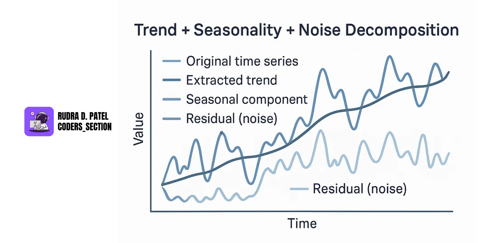
Example: A company’s revenue increasing over years.

• Seasonality: Regular patterns that repeat over a known, fixed period.

Example: More ice cream sales in summer, higher electricity usage in winter.

• Noise: Random variation that can’t be explained or predicted.

Example: Sudden drop in sales due to a one-day website outage.

7.1.2 Decomposition of Time Series

Time series decomposition breaks data into three parts:

Additive Model:

$Time Series = Trend + Seasonality + Residual (Noise)$

Multiplicative Model:

$Time Series = Trend \times Seasonality \times Residual (Noise)$

7.1.3 Forecasting Methods (ARIMA, Moving Averages)

Moving Averages (MA):

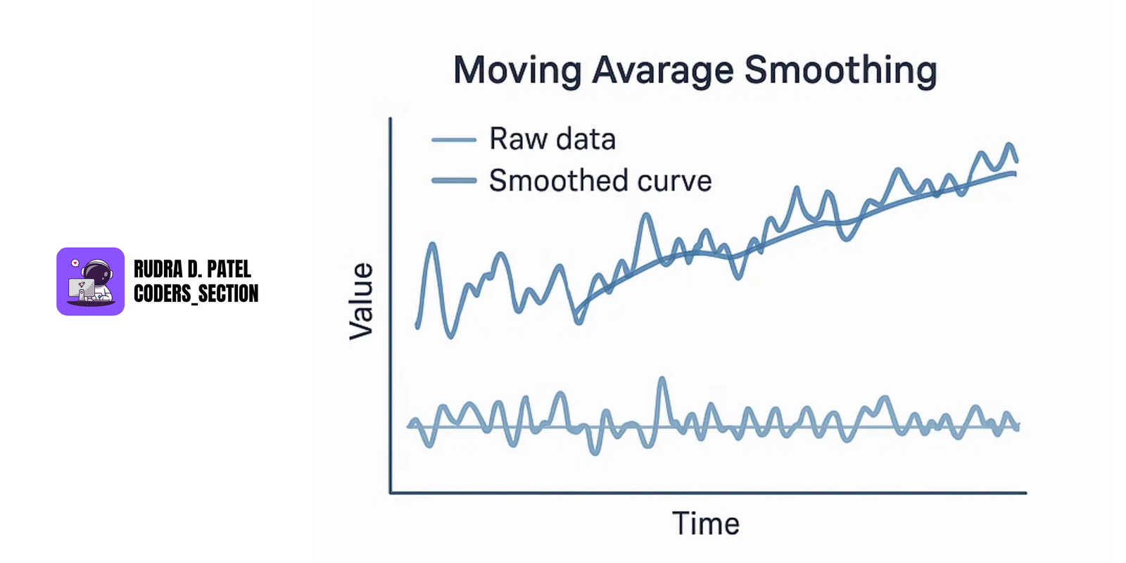
• Smooths out short-term fluctuations to highlight longer-term trends or cycles.

$SMA_t = (X_t + X_{t-1} + ... + X_{t-N+1}) / N$

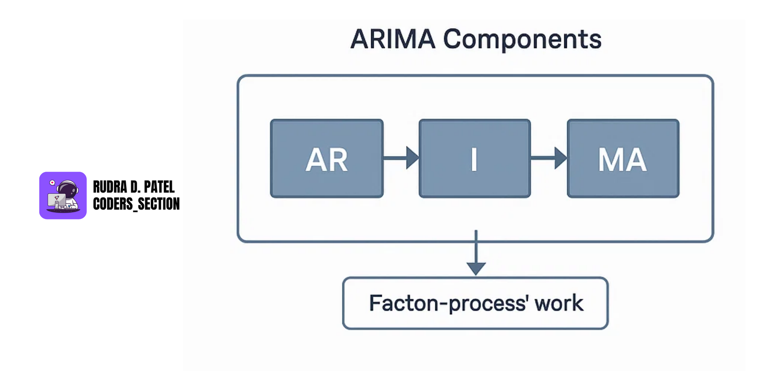
ARIMA (AutoRegressive Integrated Moving Average):

• A popular statistical method for time series forecasting.
• Combines AR (Autoregressive), I (Integrated), and MA (Moving Average) components.

7.1.4 Time-Series Cross-Validation

Unlike random splits, time series uses time-based validation:

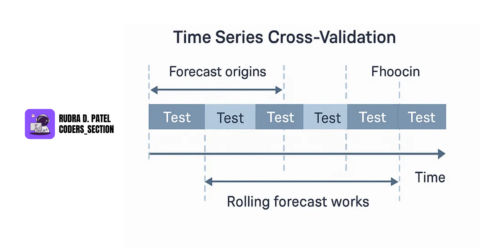
Rolling Forecast Origin (Walk-forward validation):

Train [1], Test [2]

Then a sliding window: Train [2,3], Test [4]

This approach respects time order and gives reliable forecast evaluation.

7.2 Clustering Techniques

Clustering is unsupervised learning, used to group similar data points.

7.2.1 K-Means Clustering

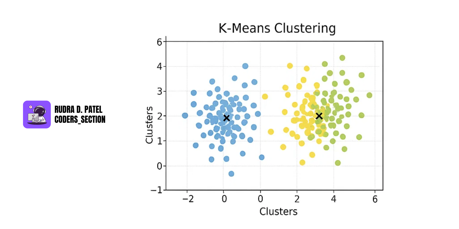
• Divides data into k groups (clusters).
• Assigns points to the cluster with the nearest centroid.
• Recalculates centroids until convergence.

Steps:

1. Choose k
2. Randomly assign centroids
3. Assign each point to nearest centroid
4. Recalculate centroids
5. Repeat until stable

Use Cases: Market segmentation, image compression, anomaly detection.

7.2.2 Hierarchical Clustering

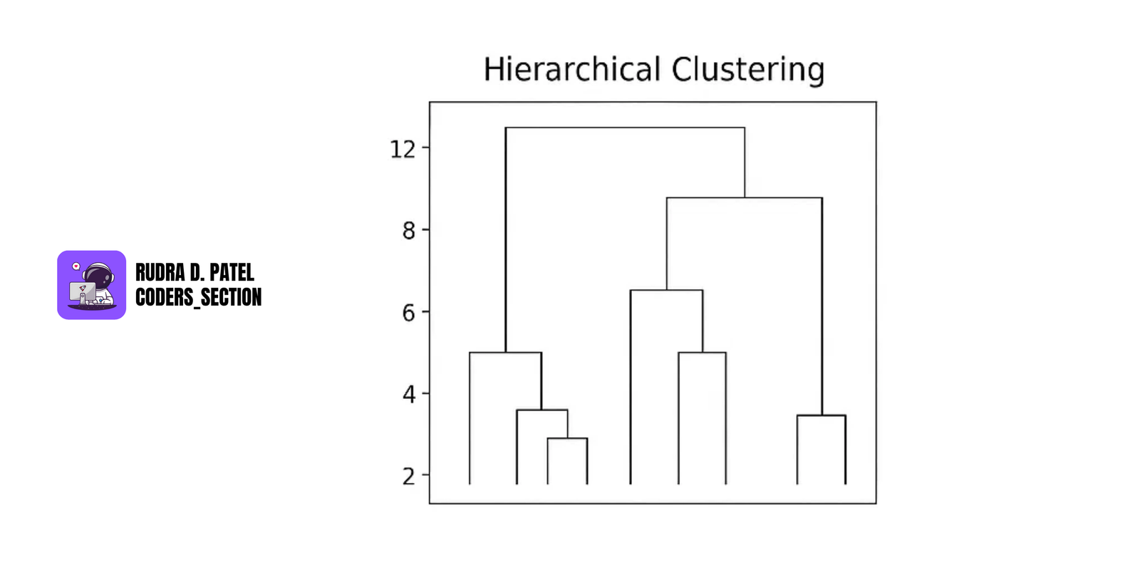
• Creates a tree-like structure (dendrogram).

Two types:

• Agglomerative: Bottom-up. Each point starts as its own cluster and clusters are merged.
• Divisive: Top-down. Starts with one cluster and splits.

No need to predefine k.

7.2.3 DBSCAN (Density-Based Spatial Clustering of Applications with Noise)

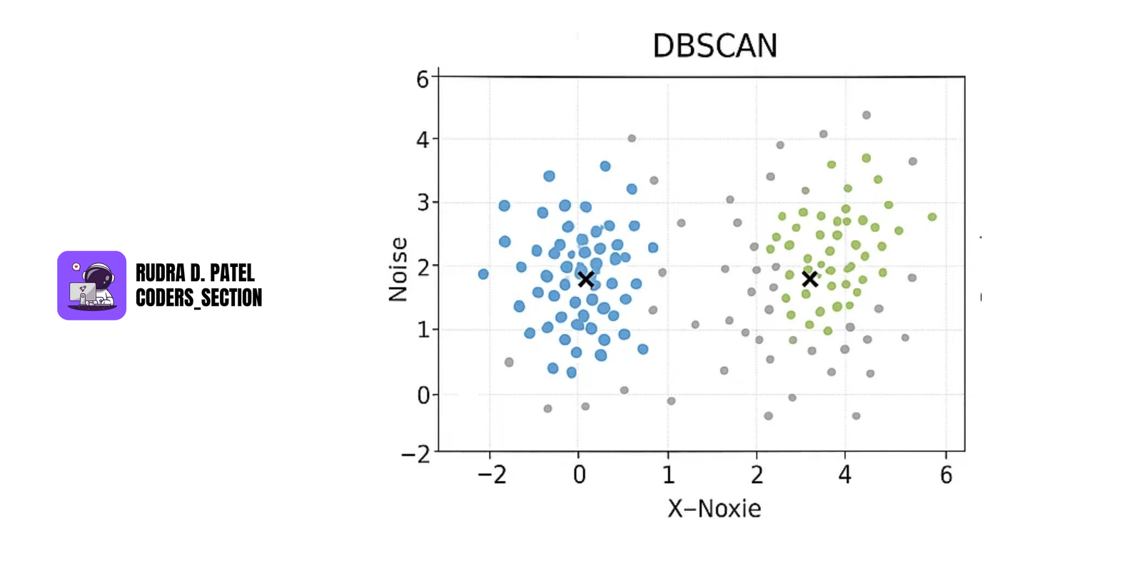
• Groups together points that are closely packed together, marking as outliers points that lie alone in low-density regions.

7.2.4 Silhouette Score and Elbow Method

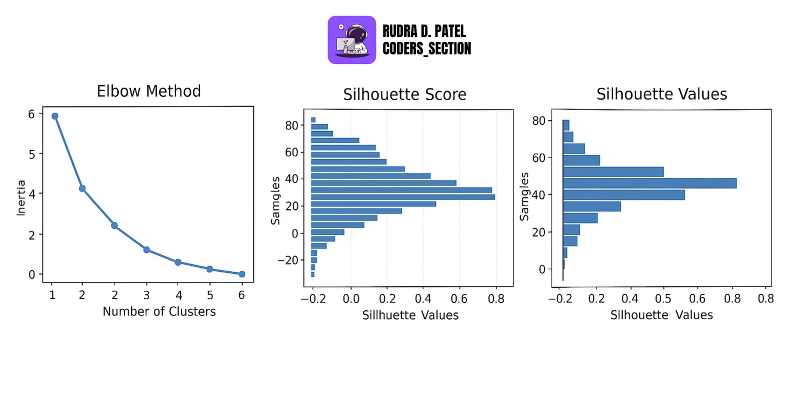
• Elbow Method: Used to find the optimal number of clusters (k) for K-Means.
• Silhouette Score: Measures how similar an object is to its own cluster compared to other clusters.

7.3 Classification and Regression Analysis

These are supervised learning techniques used to predict outcomes.

7.3.1 Decision Trees

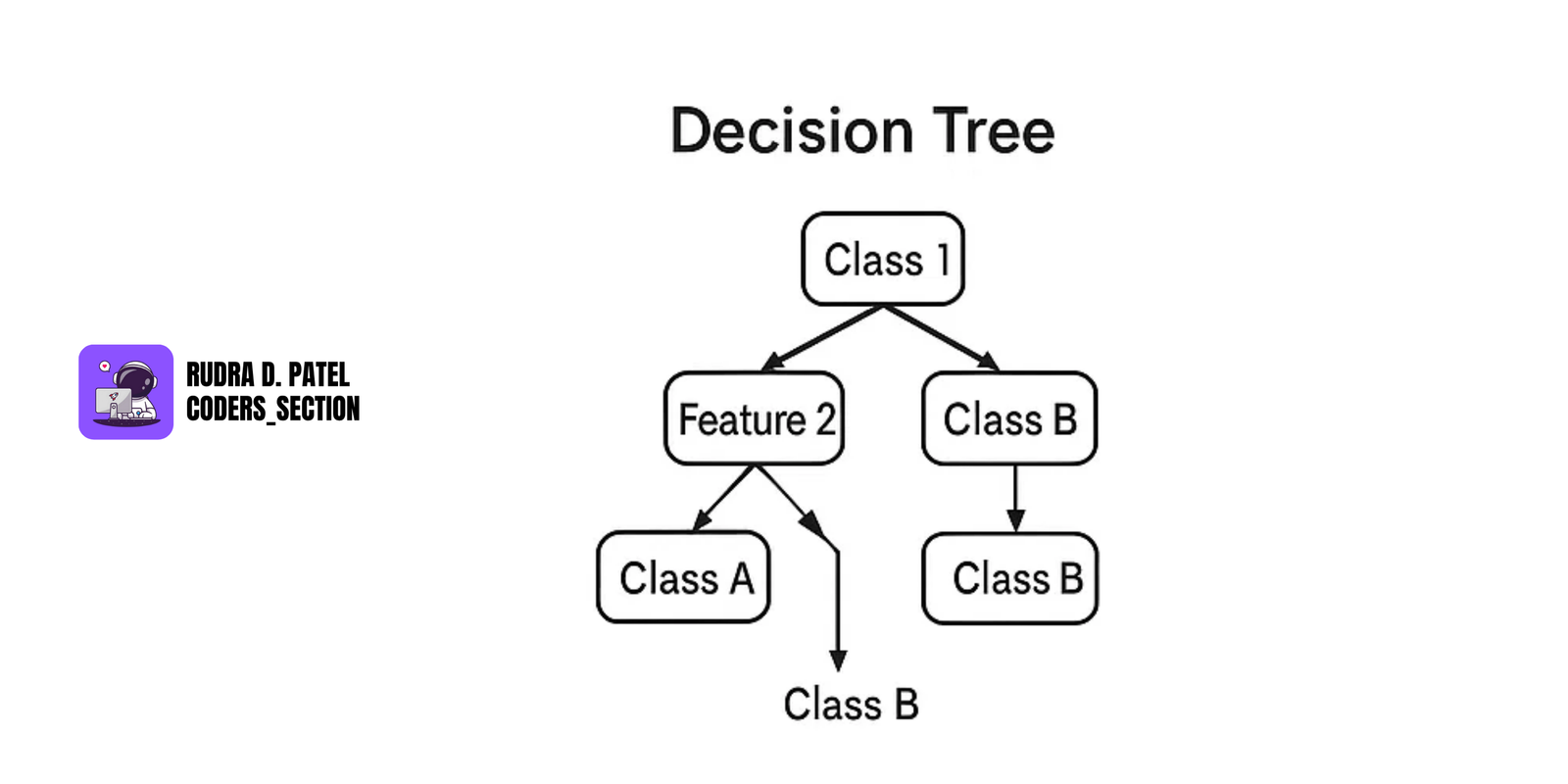
• Tree structure where each node represents a decision based on a feature.
• Splits data into subsets based on feature values.
• Leaves represent the final decision or prediction.

Pros:

• Easy to interpret
• Handles both classification and regression

7.3.2 Random Forest

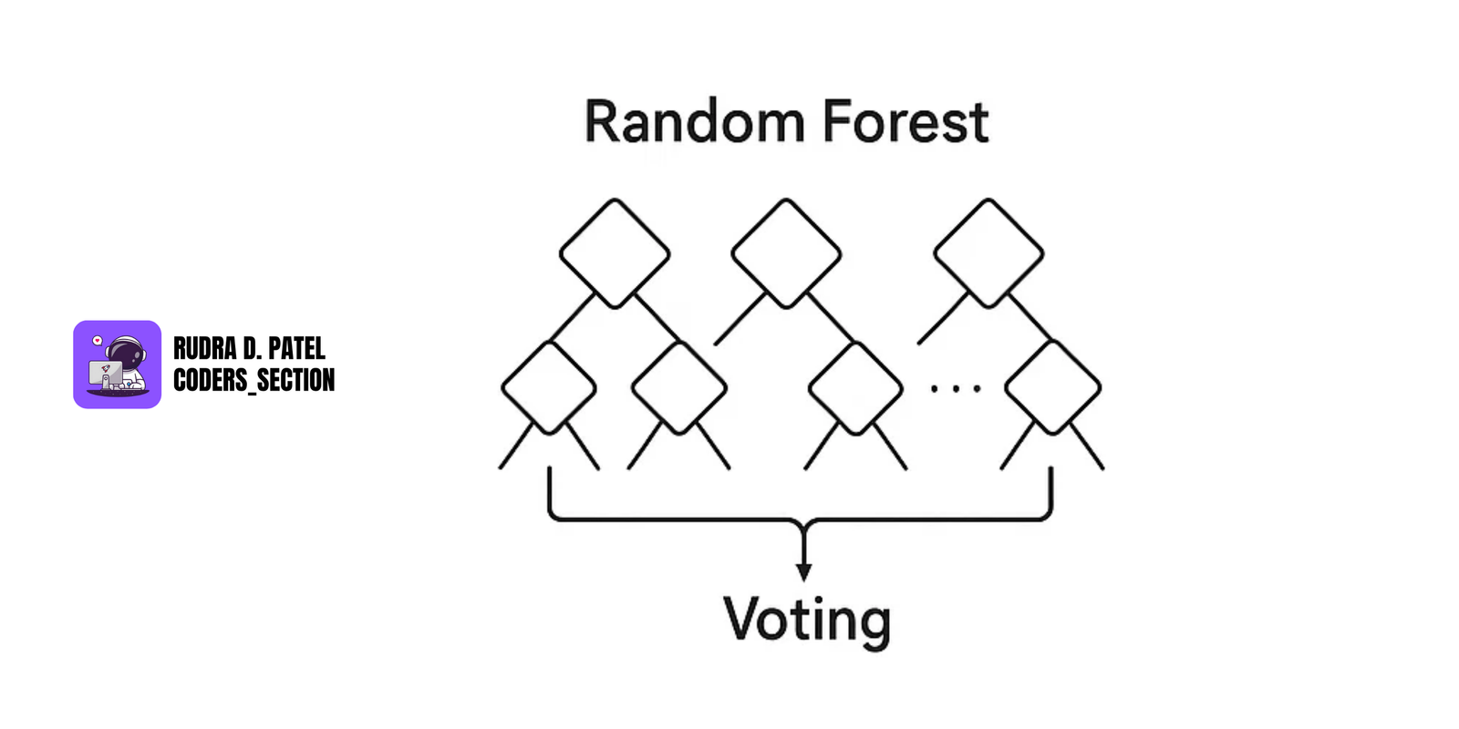
• Ensemble of multiple decision trees.
• Each tree gets a random subset of data and features.
• Combines results from all trees:
• Classification: Voting
• Regression: Averaging

Advantages:

• Reduces overfitting
• Improves accuracy

7.3.3 SVM (Support Vector Machines)

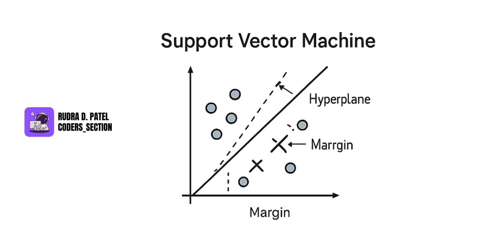
• Finds the best boundary (hyperplane) that separates classes.
• Maximizes margin between support vectors (closest points from each class).

Use for:

• Binary classification
• Text classification
• Image classification

Kernels allow it to handle non-linear data:

• Linear Kernel
• RBF Kernel
• Polynomial Kernel

7.3.4 KNN (K-Nearest Neighbors)

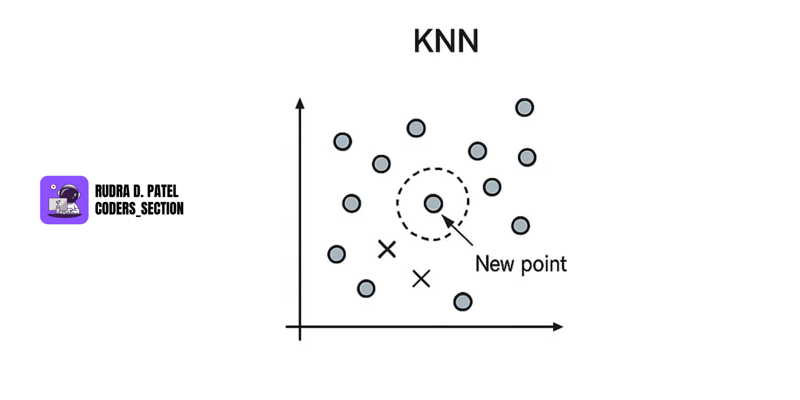
• A lazy learner — stores all training data.
• For a new data point, it finds the 'k' nearest data points in the training set.
• Classification: Assigns the class that is most common among its K nearest neighbors.
• Regression: Assigns the average value of its K nearest neighbors.

7.3.5 Naive Bayes Classifier

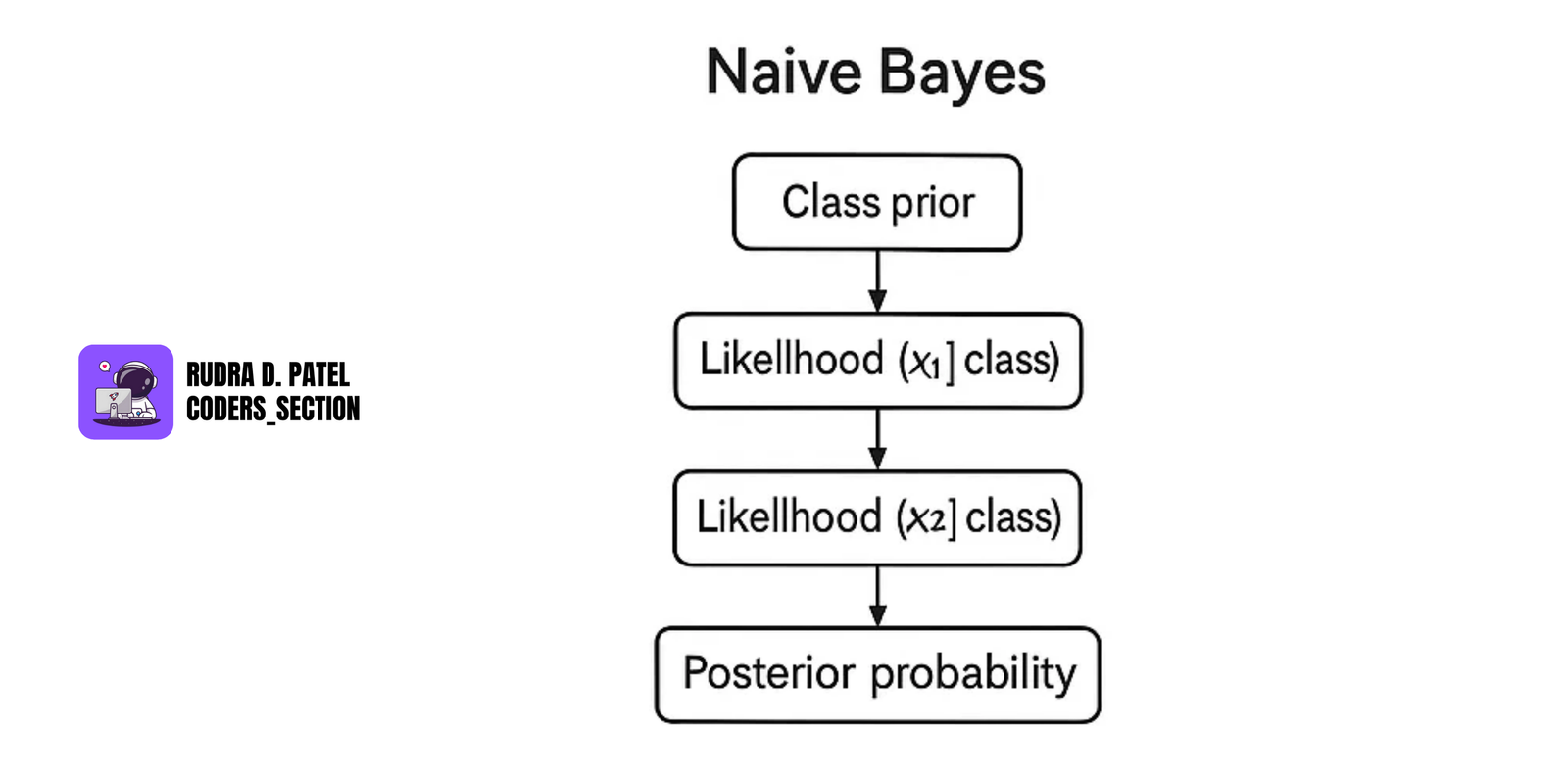
• Based on Bayes' Theorem (see Section 2.2.3).
• Assumes features are independent.

Formula:

$P(Class|Features) = P(Features|Class) \times P(Class) / P(Features)$

Use Cases: Spam detection, sentiment analysis.

7.3.6 Linear vs. Logistic Regression

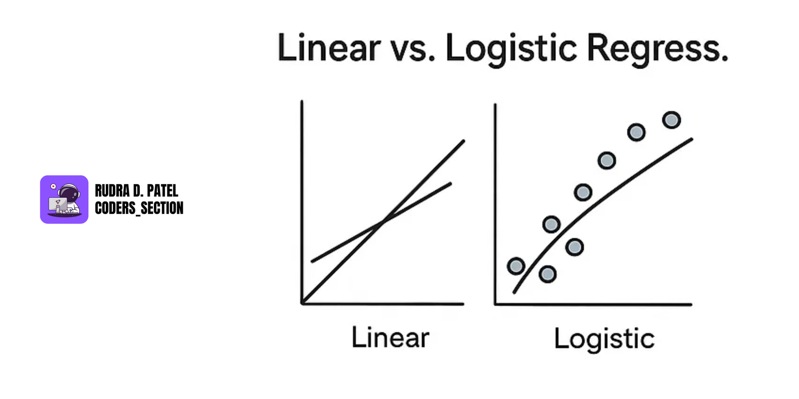
Linear Regression

• Predicts a continuous numeric value.

Formula:

$y = mx + b$

Logistic Regression

• Predicts probabilities for binary classification (e.g., 0 or 1).
• Uses sigmoid function:

$P(Y=1|X) = 1 / (1 + e^{-(mX + b)})$

Data visualization is the art of converting raw data into visual formats like graphs and charts, so insights are easier to understand and communicate. Choosing the right type of chart is key.

8.1 Designing Effective Charts

Choosing the right chart helps present data clearly and avoid confusion. Here's a breakdown:

Bar Chart

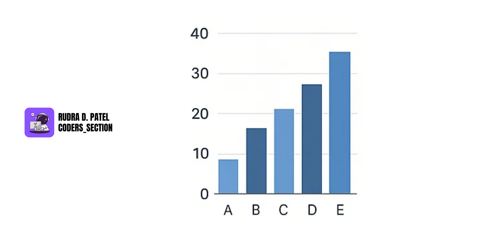
• Used to compare values across categories.
• Best when categories are distinct and few.

Example: Sales in different regions (North, South, East, West).

• Bars should be the same width and have clear labels.

Pie Chart

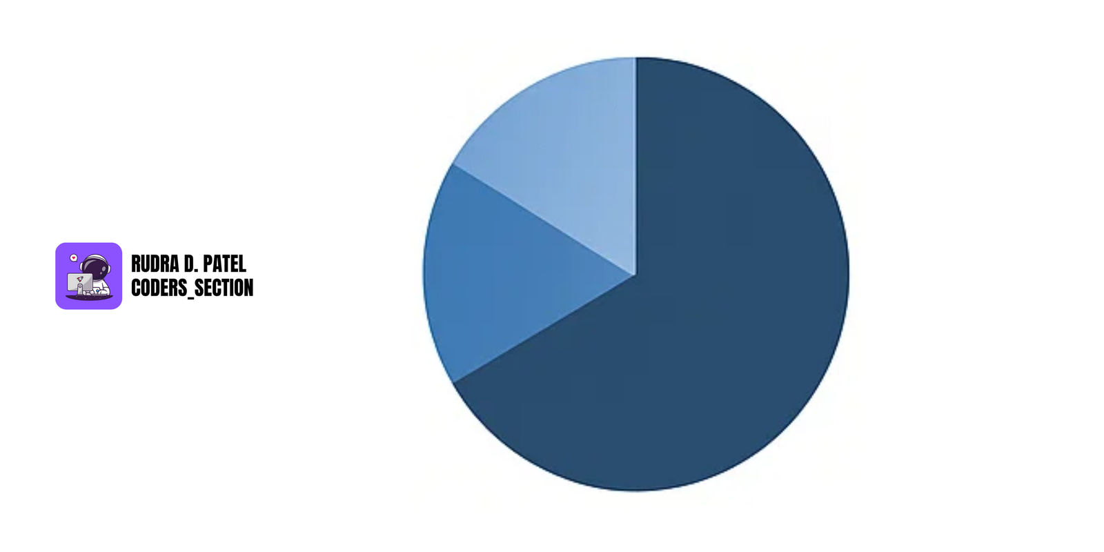
• Used to show part-to-whole relationships.
• Best when you want to highlight how a category contributes to a whole.

Example: Market share of 4 brands.

• Avoid using for more than 5 categories, as it becomes hard to read.

Line Chart

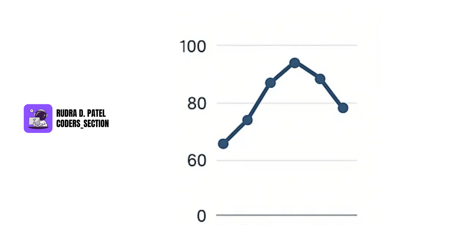
• Used to display trends over time.
• Great for time-series data like daily temperatures or stock prices.
• Connects data points with a line, making it easy to spot increases/decreases.

Histogram

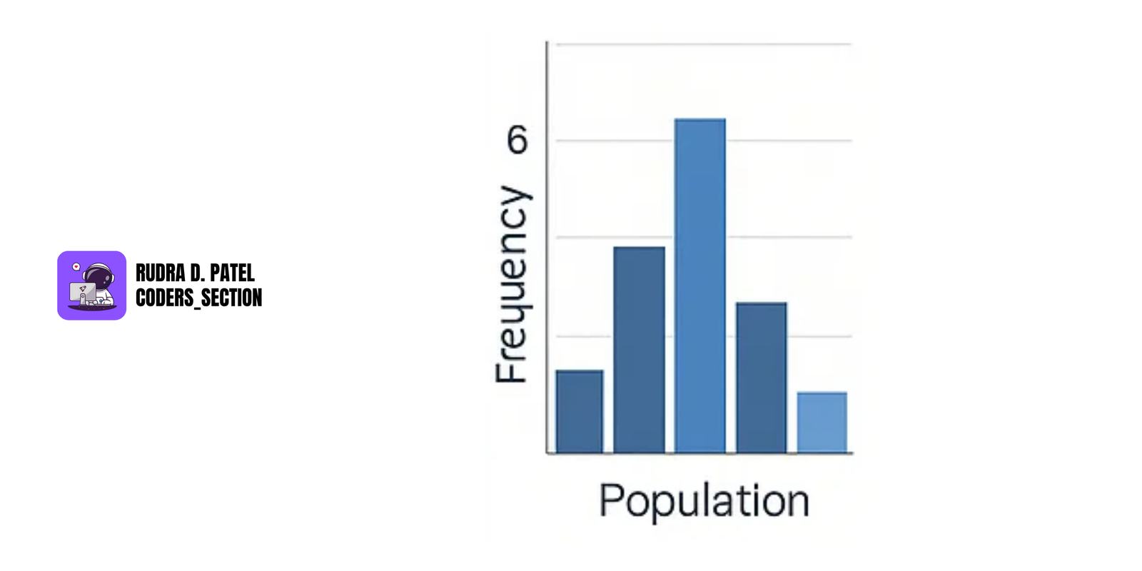
• Shows the distribution of continuous data.

Example: Age distribution of customers.

• Divides the data into bins and shows frequency in each bin.
• Helps identify data skewness, outliers, or normal distribution.

8.1.2 Visualizing Multivariate Data

Multivariate data has more than two variables.

You can use:

• Bubble charts: like scatter plots, but size of bubble adds a 3rd dimension.
• Heatmaps: show values with colors; used in correlation matrices.
• Pairplots: shows all pairwise relationships between variables (common in data analysis).

8.1.3 Visualizing Distributions and Relationships

• Use Boxplots to show median, quartiles, and outliers in a distribution.
• Violin plots show the density of the distribution.
• Scatter plots show relationships (correlations) between two continuous variables.

Example: Hours studied vs. exam score.

• Correlation heatmaps help spot strong or weak relationships between variables.

8.2 Advanced Visualization Tools

8.2.1 Python Libraries

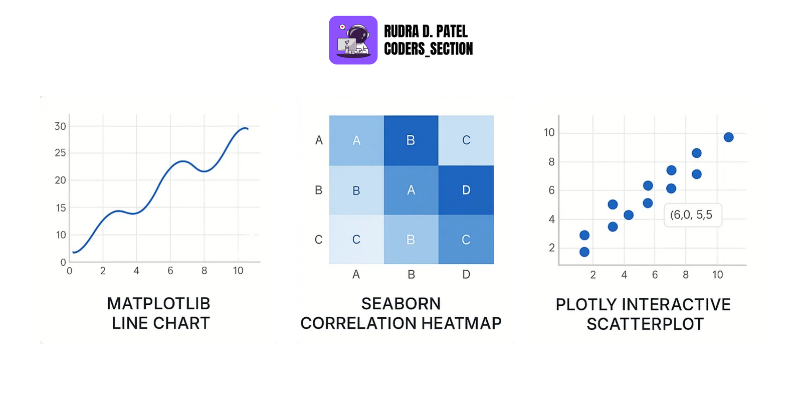
Matplotlib

• The basic plotting library in Python.
• Used to create line charts, bar charts, scatter plots, etc.
• Highly customizable for publication-ready graphs.

Seaborn

• Built on top of Matplotlib.
• Makes statistical plots look better and easier to build.
• Good for heatmaps, boxplots, violin plots, pairplots, etc.

Plotly

• Used for interactive plots in dashboards and web apps.
• Supports zoom, hover, and other user interactions.

8.2.2 Business Intelligence (BI) Tools

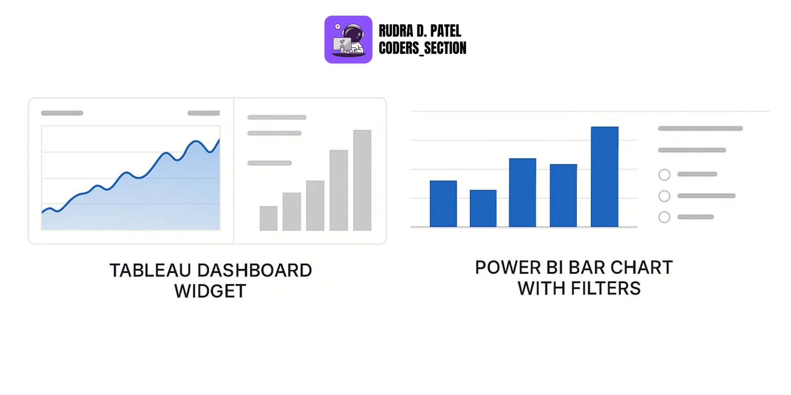
Tableau

• A leading BI tool for creating interactive dashboards and reports.
• Drag-and-drop interface makes it easy to use.

Power BI

• Microsoft’s visualization tool.
• Integrates well with Excel and other MS tools.
• Used for interactive dashboards and business reports.

8.3 Storytelling with Data

8.3.1 Creating Data-Driven Narratives

Good data visualization is not just about charts—it tells a story.

• Ask: What do I want my audience to learn from this?

Structure it like a story:

• Set the context (problem)
• Show supporting data
• Share insights
• Make a recommendation

8.3.2 Combining Data Insights with Visuals

• Use highlights, annotations, or labels to draw attention to key points.

Example: Circle a spike in sales on a line chart and explain what caused it.

• Use consistent colors and fonts.
• Keep charts simple; avoid clutter.

9.1 Communicating Results

9.1.1 Writing Data Analysis Reports

Should include:

• Objective of the analysis
• Methodology (how the data was collected/cleaned)
• Key insights
• Charts/tables for visual explanation
• Final recommendations

Keep the report:

• Clear
• Concise
• Non-technical (if for business audience)

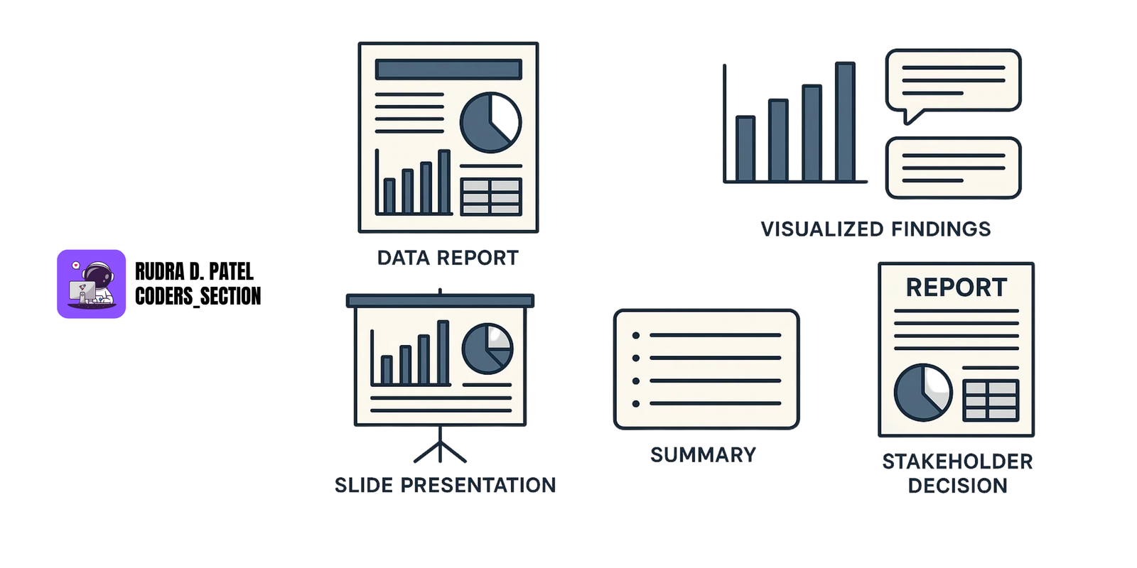
9.1.2 Presenting Findings and Insights

• Use PowerPoint, PDFs, or dashboards.
• Focus on storytelling instead of just numbers.
• Use one insight per slide/chart.
• Always explain “why” the data matters.

9.1.3 Using Visuals to Support Arguments

• Always support claims with data.

Example: If you say “Sales dropped due to seasonality,” show a line chart over 12 months proving that.

9.2 Data Interpretation

9.2.1 Identifying Key Insights and Patterns

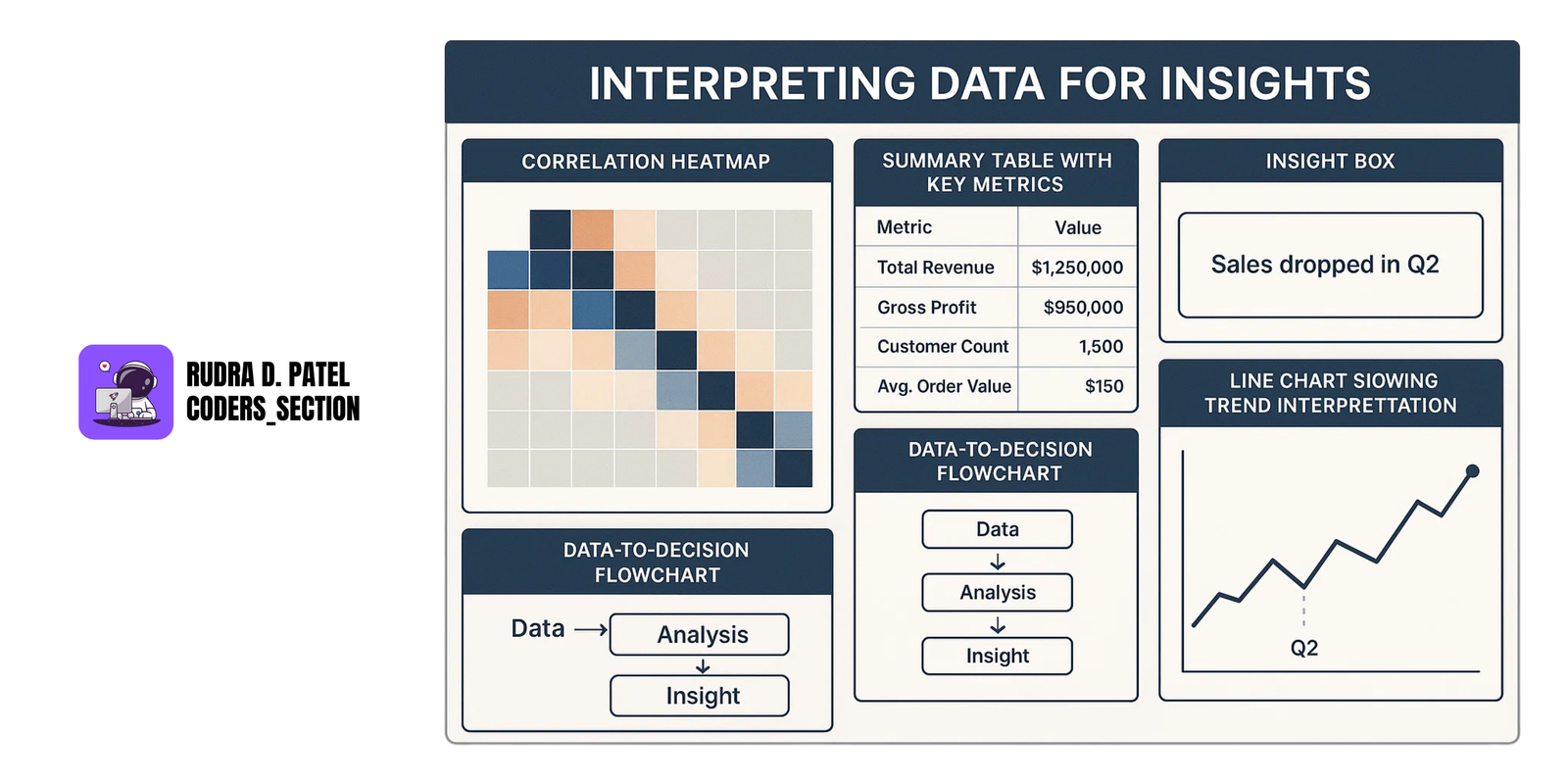
Look for:

• Trends (e.g., increasing sales)
• Patterns (e.g., weekly traffic spikes)
• Anomalies (e.g., sudden drop in users)

• Use summary statistics (mean, median) and charts to help spot these.

9.2.2 Drawing Conclusions from Data

• Translate findings into actionable insights.
• Don’t just say “Sales dropped in Q2.” Explain why, and what to do next.

9.2.3 Making Data-Driven Decisions

• The ultimate goal of data analysis is to enable better decision-making.
• Ensure your insights are clear, actionable, and supported by evidence.

10.1 Python for Data Analysis

Python is one of the most popular languages in data analysis because of its simplicity and powerful libraries. Here's what you need to know:

10.1.1 Pandas

• A library used for working with structured data (tables).

Key features:

• DataFrame and Series for storing data.
• Easy to read CSV, Excel, JSON files.
• Functions for filtering, grouping, merging, reshaping data.

10.1.2 NumPy

• Stands for Numerical Python.
• Provides support for multi-dimensional arrays and matrices.

Useful for:

• Mathematical operations
• Linear algebra, random number generation, statistics

10.1.3 Matplotlib

• A basic plotting library in Python.
• Used to create line charts, bar charts, scatter plots, etc.
• Highly customizable for publication-ready graphs.

10.1.4 Seaborn

• Built on top of Matplotlib.
• Makes statistical plots look better and easier to build.
• Good for heatmaps, boxplots, violin plots, pairplots, etc.

10.1.5 Plotly

• Used for interactive plots in dashboards and web apps.
• Supports zoom, hover, and other user interactions.

10.1.6 SciPy, Statsmodels

• SciPy: Scientific computing library for Python (optimization, integration, interpolation).
• Statsmodels: Provides classes and functions for the estimation of many different statistical models.

10.1.7 Jupyter Notebooks for Interactive Analysis

• Web-based interactive computing environment for creating and sharing documents containing live code, equations, visualizations, and narrative text.

10.2 R for Data Analysis

R is a language designed specifically for statistical computing and graphics.

10.2.1 dplyr

• Part of the tidyverse.
• Used for data manipulation: filtering, selecting, mutating, summarizing.
• Syntax like `filter()`, `select()`, `group_by()`, `summarize()`.

10.2.2 ggplot2

• Most popular data visualization library in R.
• Based on the Grammar of Graphics.
• Allows creation of high-quality graphs and plots with minimal code.

10.2.3 tidyr

• Helps in tidying messy data (e.g., from wide to long format).
• Functions like `pivot_longer()` and `pivot_wider()` make reshaping easy.

10.2.4 caret

• Stands for Classification and Regression Training.
• Used for machine learning workflows.
• Handles preprocessing, model training, and evaluation.

10.2.5 RMarkdown

• Combine code, analysis, and report writing in one file.
• Export to HTML, PDF, or Word.
• Very useful for automated reports and documentation.

10.3 Excel for Data Analysis

Excel is still widely used in businesses due to its simplicity and accessibility.

10.3.1 Pivot Tables

• Summarize and analyze large datasets, allowing for quick aggregation and cross-tabulation.

10.3.2 Excel Formulas and Functions

• SUM, AVERAGE, COUNT, IF, VLOOKUP, INDEX/MATCH for data manipulation and analysis.

10.3.3 Data Analysis ToolPak

• An Excel add-in that provides statistical analysis tools (e.g., regression, ANOVA, descriptive statistics).

10.4 SQL for Data Analysis

SQL (Structured Query Language) is used to extract and manipulate data from databases.

10.4.1 SQL Queries

• SELECT, FROM, WHERE are the building blocks of SQL.
• You use them to retrieve specific data based on conditions.

10.4.2 JOIN Operations

• Used to combine data from multiple tables.

Common joins:

• INNER JOIN
• LEFT JOIN
• RIGHT JOIN
• FULL OUTER JOIN

10.4.3 Aggregations and Grouping

• Functions like SUM(), AVG(), COUNT(), MAX(), MIN().
• Group data using GROUP BY to analyze by category.

10.4.4 Window Functions

• Perform calculations across a set of rows related to the current row.

Examples:

• ROW_NUMBER() – assigns rank to each row.
• RANK() – shows position of a row based on a column.
• LEAD() and LAG() – access previous or next row value.

Machine Learning helps data analysts build models that learn from data and make predictions or discover patterns. It's a core part of modern data analysis and business intelligence.

11.1 Supervised Learning Techniques

Supervised Learning is when we train a model on labeled data—data that has input and the correct output.

11.1.1 Regression Models

• Used when the output is a continuous value, like predicting temperature, prices, or sales.

Linear Regression

• Predicts a value based on a linear relationship.

Example: Predicting house price based on area.

Logistic Regression

• Used when the target is binary (yes/no, 0/1).

Example: Predicting if an email is spam or not.

11.1.2 Classification Models

• Used when the output is a category or class (e.g., high/low, yes/no, red/blue).

Decision Trees

• A flowchart-like structure that splits data based on conditions.
• Easy to understand and interpret.

Random Forest

• A collection of multiple decision trees (ensemble).
• More accurate and less prone to overfitting.

11.1.3 SVM (Support Vector Machines)

• Finds the best boundary (hyperplane) that separates classes.

11.1.4 KNN (K-Nearest Neighbors)

• Classifies a data point based on the majority class of its 'k' nearest neighbors.

11.1.5 Naive Bayes Classifier

• A probabilistic classifier based on Bayes' theorem with strong independence assumptions between features.

11.2 Unsupervised Learning

Unsupervised Learning is when we train a model on unlabeled data—data without predefined output labels. The goal is to find hidden patterns or structures.

11.2.1 Clustering Methods (K-Means, DBSCAN)

• K-Means: Groups data into 'k' clusters based on similarity.
• DBSCAN: Groups data points that are closely packed together, marking as outliers points that lie alone in low-density regions.

11.2.2 Dimensionality Reduction (PCA)

• PCA (Principal Component Analysis): Reduces the number of features in a dataset while retaining most of the variance.

11.3 Model Evaluation and Metrics

After building a model, we need to evaluate its performance using proper metrics.

11.3.1 Accuracy, Precision, Recall, F1-Score

• Accuracy = Correct Predictions / Total Predictions
• Used when classes are balanced.
• Precision = Correct Positives / All Predicted Positives
• Used when false positives are costly (e.g., spam filter).
• Recall = Correct Positives / All Actual Positives
• Used when false negatives are costly (e.g., disease detection).
• F1-Score = Harmonic Mean of Precision and Recall
• Used when we want a balance between precision and recall.

11.3.2 Cross-Validation and Hyperparameter Tuning

Cross-Validation

• Splits the data into multiple parts to test model performance more reliably.
• Helps avoid overfitting.

Hyperparameter Tuning

• Fine-tunes the model's settings (e.g., tree depth, learning rate) to improve accuracy.

11.3.3 Confusion Matrix and ROC-AUC

Confusion Matrix

• A table showing actual vs. predicted outcomes.
• Helps you see where the model is making errors (TP, FP, TN, FN).

ROC-AUC (Receiver Operating Characteristic - Area Under Curve)

• Evaluates the performance of classification models across all classification thresholds.
• Higher AUC indicates better model performance.

These projects show how various data analysis techniques are used in real-life scenarios. Each project covers a different type of analysis and tool.

12.1 Exploratory Data Analysis (EDA) on Sales Data

• Goal: Understand overall sales performance, trends, and product/customer behavior.

Steps:

• Import sales data from Excel/CSV.
• Clean data (handle missing values, fix data types).
• Use Pandas and Seaborn to:
• Analyze total revenue, monthly sales trends, best-selling products.
• Visualize with bar charts, line plots, pie charts.
• Use pivot tables or groupby() to:
• Compare sales by category, region, or salesperson.

Tools Used:

• Python (Pandas, Matplotlib, Seaborn)
• Excel for quick pivoting
• Jupyter Notebook for reporting

12.2 Customer Segmentation using K-Means Clustering

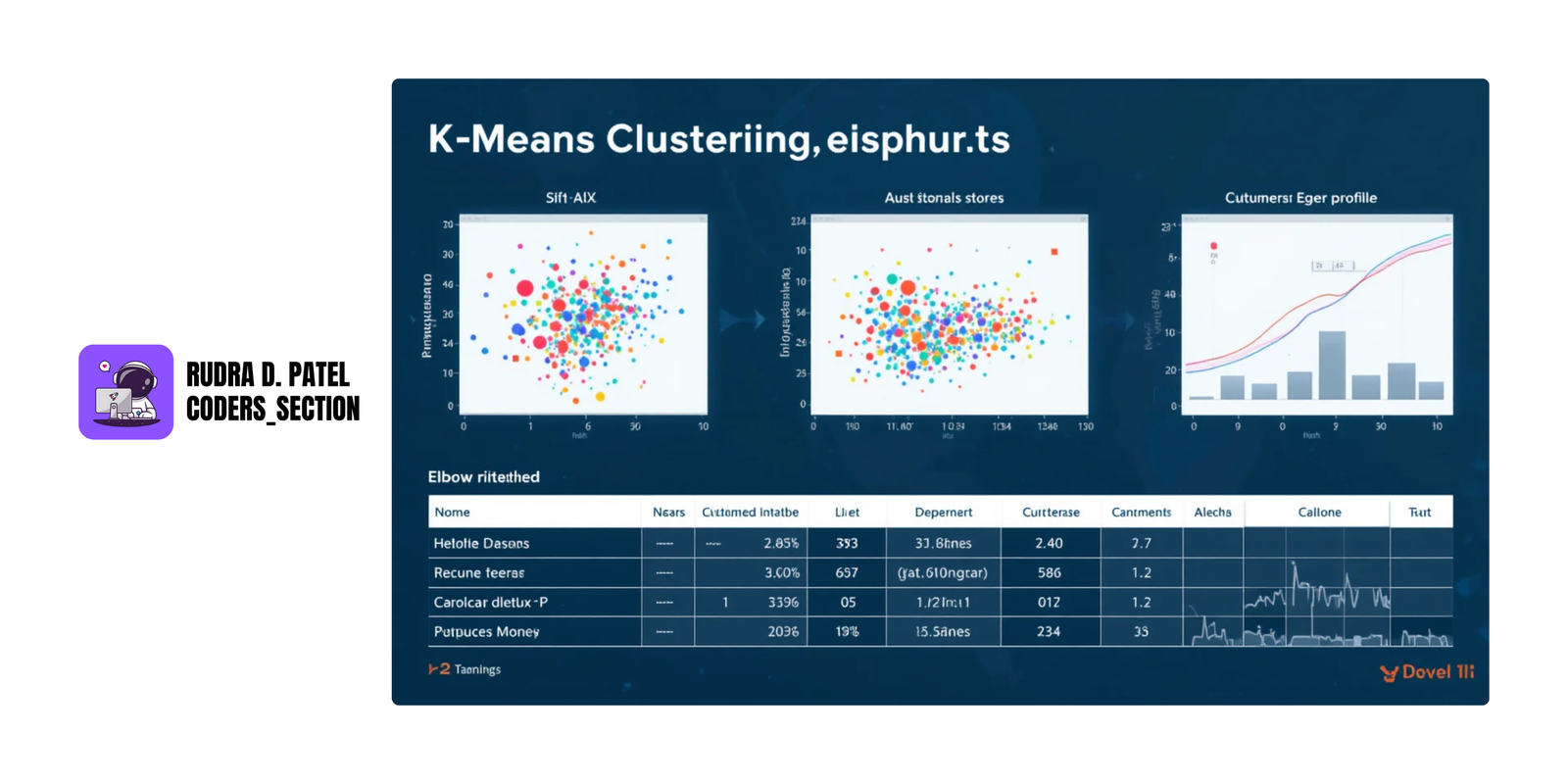
• Goal: Group customers into clusters based on buying behavior to improve marketing strategies.

Steps:

• Use customer data: age, annual income, spending score, etc.
• Standardize data using scaling techniques.
• Apply K-Means clustering to find optimal customer groups.
• Visualize clusters using scatter plots.

Outcome:

• Identify different customer segments (e.g., high-value, budget-conscious) for targeted campaigns.

Tools Used:

• Python (Scikit-learn, Pandas, Matplotlib)
• Jupyter Notebook for explanations

12.3 Predicting Housing Prices using Regression

• Goal: Build a model to predict house prices based on features like area, number of rooms, and location.

Steps:

• Collect housing dataset.
• Perform EDA to understand feature relationships.
• Split data into training and testing sets.
• Build a Linear Regression model.
• Evaluate model using R-squared, Mean Squared Error (MSE).

Outcome:

• Provide estimated house prices for new properties.

Tools Used:

• Python (Scikit-learn, Pandas)
• Jupyter Notebook for explanations

12.4 Analyzing Stock Market Trends using Time-Series

• Goal: Analyze stock prices over time and forecast future values.

Steps:

• Collect historical stock data (e.g., from Yahoo Finance).
• Use line plots to visualize daily/weekly prices.
• Decompose data into trend, seasonality, and noise.
• Apply Moving Averages, ARIMA, or Prophet for forecasting.
• Use cross-validation to check accuracy.

Tools Used:

• Python (Pandas, Statsmodels, ARIMA, Prophet)
• Matplotlib, Seaborn for charts

12.5 Classifying Customer Churn using Logistic Regression

• Goal: Predict whether a customer will stop using the service (churn) or not.

Steps:

• Load telecom or subscription dataset.
• Convert categorical features using encoding.
• Build a Logistic Regression model.
• Evaluate model using Accuracy, Confusion Matrix, ROC-AUC.
• Identify key features that influence churn.

Outcome:

• Help businesses reduce customer loss and improve retention strategies.

Tools Used:

• Python (Scikit-learn, Pandas)
• Jupyter Notebook for explanations

Understanding ethics is crucial in data analysis. Data can be powerful, but with power comes responsibility. Analysts must ensure that data is handled fairly, securely, and without bias.

13.1 Data Privacy and Security

13.1.1 GDPR and Data Protection

• GDPR (General Data Protection Regulation) is a law in the EU that protects personal data of individuals.

It gives people rights like:

• Right to know how their data is used.
• Right to delete their data.
• Right to consent before collecting data.

If you collect or analyze data from users, you must:

• Get permission (consent).
• Tell them why and how you’re using the data.
• Store it safely and protect it from breaches.

Example: If you collect email addresses for analysis, you must tell users and secure that data using encryption.

13.1.2 Ethical Use of Personal Data

• Never use personal data for purposes other than what was agreed.
• Avoid selling or sharing data without permission.
• Anonymize sensitive information before using it in reports or models.
• Follow "data minimization" (collect only what's necessary).

13.2 Bias in Data

13.2.1 Identifying and Mitigating Bias

• Bias can creep into data collection and analysis, leading to unfair or inaccurate results.

Examples of bias:

• Selection bias: Data collected from a non-representative group.
• Confirmation bias: Interpreting data to support existing beliefs.

Mitigation:

• Ensure diverse data sources.
• Use fair sampling methods.
• Regularly audit data for imbalances.

13.2.2 Fairness in Data Analysis and Models

• Ensure that your models do not discriminate against certain groups.
• Test models for fairness across different demographic segments.
• Be transparent about data limitations and potential biases.