1. INTRODUCTION TO DATA SCIENCE
1.1 What is Data Science?
Basic Definition:
- Data Science is the study and practice of extracting knowledge and insights from data. It uses math, coding, and domain understanding to solve real-world problems.
- You can think of it like this: "You collect data → You understand the data → You find patterns → You use those patterns to make smart decisions."
In Simple Terms:
Data Science is a combination of:
- Statistics - to understand numbers and trends
- Programming - to write code and work with data
- Visualization - to create graphs and charts
- Domain Knowledge - to understand the problem you're solving
Real-Life Example:
Let's say you own a small shop.
- You write down what you sell every day in a notebook.
Over time, this notebook becomes:
- A source of data (your sales)
- With that data, you can ask questions like:
- What is my best-selling product?
- On which days do I sell the most?
- When should I give discounts?
- Answering these questions using your data = Data Science.
Why is it Important?
- It helps companies make better decisions
- It helps predict the future
- It helps to find problems early
- It improves customer experience
1.2 Data Science Workflow
The Data Science workflow is a set of steps that every data scientist follows to solve a problem using data.
Let's understand each step like you're solving a school project.
Step 1: Problem Understanding
You must understand:
- What is the goal?
- What are we trying to find out?
Example: "Why are customers uninstalling our app?"
1.2 Data Science Workflow (continued)
Step 2: Data Collection
- This means gathering the data from different places.
Sources of data:
- Databases (like MySQL, MongoDB)
- Excel/CSV files
- Web scraping (getting data from websites)
- APIs (data from services like weather, maps)
Example: Get data about user logins, actions, purchases, feedback.
Step 3: Data Cleaning (Preprocessing)
- Raw data is often messy.
- This step is about making it correct and usable.
Common cleaning tasks:
- Removing duplicates
- Filling missing values
- Fixing typos or wrong formats
- Removing outliers (very large or very small values)
Example: If someone's age is written as 400 - that needs to be fixed.
Step 4: Data Exploration (EDA - Exploratory Data Analysis)
- You now look at the data to understand it better.
This includes:
- Basic statistics (mean, median, mode)
- Graphs (bar chart, pie chart, line chart)
- Finding patterns and trends
Example: More users uninstall the app after 10 PM this might mean poor late-night support.
Step 5: Data Modeling
- Here, you use Machine Learning or statistical models to make predictions or classifications.
Types of models:
- Linear Regression (predict numbers)
- Decision Trees (classify options)
- Clustering (grouping similar items)
Example: Predict if a new user will uninstall the app in 7 days.
1.2 Data Science Workflow (continued)
Step 6: Evaluation
- Check how well your model is performing.
Use:
- Accuracy
- Precision and Recall
- Confusion Matrix
Example: Your model is 80% accurate this means it correctly predicted 8 out of 10 cases.
Step 7: Communication (Visualization & Reporting)
- Now it's time to present your findings.
You can use:
- Charts (bar, line, scatter, heatmaps)
- Dashboards (in tools like Power BI or Tableau)
- Reports (slides or PDF summaries)
Example: Show a graph that uninstall rates are high on weekends, and give suggestions.
1.3 Roles & Responsibilities of a Data Scientist
A Data Scientist is someone who works with data to help people or businesses make better decisions.
They are problem-solvers who use data to:
- Understand what is happening
- Find out why it's happening
- Predict what might happen next
Main Roles & Tasks:
- Ask the Right Questions
- Understand the business goal
- Define what problem needs to be solved
- Collect Data
- From different sources like SQL, Excel, APIs
- Ensure the data is reliable
- Clean the Data
- Fix missing or incorrect values
- Make the data ready for use
- Explore the Data
- Find patterns, trends, and relationships
- Use visualizations to understand better
- Build Models
- Use ML or statistical models
- Train and test the model on real data.
1.3 Roles & Responsibilities of a Data Scientist (continued)
- Evaluate Models
- Check how well the model is working
- Improve or try different models if needed
- Present Insights
- Use graphs and dashboards
- Explain in simple language what the data shows
Skills a Data Scientist Needs:
- Programming (Python or R)
- Statistics & Math
- Data Handling (Pandas, SQL)
- Machine Learning
- Visualization (Matplotlib, Seaborn, Power BI, Tableau)
- Communication Skills
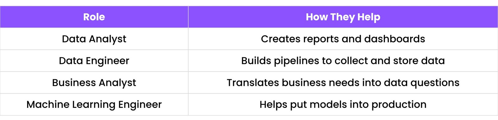
Who Do They Work With?
2. PYTHON FOR DATA SCIENCE
2.1 Python Basics: Syntax, Variables, Data Types
What is Python?
- Python is a programming language that is easy to read and write.
It's widely used in data science because:
- It's beginner-friendly
- It has powerful libraries for data
- It looks like plain English
Syntax (How Python Code Looks)
- Syntax means rules of how code should be written.
Example:
print("Hello, World")
- No semicolons at the end of lines
- Indentation (spaces) is used to define blocks of code
- Case-sensitive - `Name` and `name` are different
Variables
- A variable is like a box that stores information.
Example:
name = "Rudra"
age = 19
Here:
- `name` is a variable storing the text "Rudra"
- `age` stores the number 19
You can change a variable anytime:
age = 20
Data Types
- Python has different types of data:
![A table showing Python data types: Integer (e.g., 10), Float (e.g., 10.5), String (e.g., 'Hello'), Boolean (True/False), List (e.g., [1, 'a', True]), Dictionary (e.g., {'key': 'value'})](Resources/Cheatsheet/Images/DataSci/2.1 - DataSci CS.jpeg)
2.2 Loops, Conditionals, and Functions
Conditionals
- Used to make decisions in code.
- They check if something is True or False.
Example:
age = 18
if age >= 18:
    print("You are an adult")
else:
    print("You are a minor")
Loops
- Loops help you repeat code.
For loop:
for i in range(5):
    print(i)
Output:
0
1
2
3
4
While loop:
count = 0
while count < 3:
    print("Hi")
    count += 1
Functions
- A function is a block of code you can reuse.
Example:
def greet(name):
    print("Hello " + name)

greet("Rudra")
Functions make code shorter and cleaner.
2.3 List Comprehensions
List comprehension is a shorter way to create lists.
Without list comprehension:
squares = []
for i in range(5):
    squares.append(i * i)
With list comprehension:
squares = [i * i for i in range(5)]
This line does the same work in one line. It’s faster and looks cleaner.
More examples:
evens = [x for x in range(10) if x % 2 == 0]
2.4 Useful Libraries: NumPy, Pandas, Matplotlib, Seaborn
Libraries are ready-made tools in Python that help you do tasks faster.
NumPy (Numerical Python)
- Used for math, arrays, and numbers.
Example:
import numpy as np
a = np.array([1, 2, 3])
print(a.mean()) # Output: 2.0
Key Features:
- Arrays (like a list but faster)
- Math operations
- Linear algebra
Pandas
- Used for data tables (rows and columns), like Excel.
Example:
import pandas as pd
data = pd.DataFrame({
    "Name": ["Rudra", "Ravi"],
    "Score": [90, 85]
})
print(data.head())
Key Features:
- Read data from CSV, Excel
- Filter, sort, clean data
- Handle missing data
Matplotlib
- Used to make basic graphs like line charts and bar charts.
Example:
import matplotlib.pyplot as plt
plt.plot([1, 2, 3], [4, 5, 6])
plt.show()
Seaborn
- Used for beautiful and advanced graphs (built on top of Matplotlib).
Example:
import seaborn as sns
sns.barplot(x=["A", "B"], y=[10, 20])
plt.show()
Key Features:
- Easy to use
- Looks better than plain Matplotlib
- Useful for data exploration
3. DATA MANIPULATION WITH PANDAS
Pandas is a powerful Python library for working with structured data (like tables with rows and columns). It helps you to:
- Analyze data
- Clean data
- Filter data
- Modify data easily
3.1 Series and DataFrame
Series
- A Pandas Series is like a single column of data.
Example:
import pandas as pd
numbers = pd.Series([10, 20, 30])
print(numbers)
Output:
0    10
1    20
2    30
dtype: int64
- It has index numbers on the left (0, 1, 2)
- And values on the right (10, 20, 30)
DataFrame
- A DataFrame is like a whole Excel sheet — a table with rows and columns.
Example:
df = pd.DataFrame({
    "Name": ["Rudra", "Ravi"],
    "Score": [90, 85]
})
print(df)
Output:
    Name  Score
0  Rudra     90
1   Ravi     85
3.2 Indexing, Slicing, Filtering
Indexing
- Use `.loc[]` and `.iloc[]` to access rows.
- `.loc[]` uses label/index name
- `.iloc[]` uses row number
Example:
print(df.loc[0]) # Row with label 0
print(df.iloc[1]) # Row at position 1
Accessing columns:
print(df["Score"]) # Selects 'Score' column
Slicing
- You can select a portion of the data using slicing.
Example:
print(df[0:1]) # Rows from 0 up to (but not including) 1
Filtering
- Use conditions to filter rows.
Example:
filtered_df = df[df["Score"] > 85]
print(filtered_df)
Output:
    Name  Score
0  Rudra     90
3.3 GroupBy and Aggregations
GroupBy
- `groupby()` is used to group rows by a column and then apply a function.
Example:
df = pd.DataFrame({
    "Class": ["A", "B", "A", "B"],
    "Marks": [85, 90, 75, 80]
})
grouped = df.groupby("Class")["Marks"].mean()
print(grouped)
Output:
Class
A    80.0
B    85.0
Name: Marks, dtype: float64
Here:
- Students are grouped by class
- Then their average marks are calculated
Aggregations
Functions like:
- `.sum()`
- `.mean()`
- `.count()`
- `.max()`, `.min()`
Example:
total_marks = df["Marks"].sum()
3.4 Merging, Joining, and Concatenation
You often need to combine different tables.
Merging
- Like SQL joins.
- You combine two DataFrames based on a common column.
Example:
students = pd.DataFrame({
    "ID": [1, 2],
    "Name": ["Rudra", "Ravi"]
})
scores = pd.DataFrame({
    "ID": [1, 2],
    "Score": [90, 85]
})
merged = pd.merge(students, scores, on="ID")
print(merged)
Output:
   ID   Name  Score
0   1  Rudra     90
1   2   Ravi     85
Joining
- Uses index instead of column.
- Usually works with `.join()` function.
Concatenation
- Used to stack multiple DataFrames together.
Example (Row-wise):
df1 = pd.DataFrame({"A": [1, 2]})
df2 = pd.DataFrame({"A": [3, 4]})
result = pd.concat([df1, df2])
print(result)
Output:
   A
0  1
1  2
0  3
1  4
3.5 Handling Missing Data
Real-world data often has missing or null values.
Detect Missing Data
df.isnull() # Shows True for missing
df.isnull().sum() # Count of missing values per column
Drop Missing Values
df.dropna() # Removes rows with any missing value
Fill Missing Values
df.fillna(0) # Fills missing with 0
df.fillna(df["Column"].mean()) # Fills with column's mean (average)
You can also use:
df["Column"].fillna(df["Column"].median()) # Fills with median
df["Column"].fillna(df["Column"].mode()[0]) # Fills with mode
4. DATA VISUALIZATION
Data Visualization is the process of turning numbers into pictures. This makes it easier to:
- See patterns
- Identify trends
- Gain insights
In Python, the most popular libraries used are:
- Matplotlib – for basic charts
- Seaborn – for more advanced and beautiful charts
Let’s go step by step:
4.1 Line, Bar, Pie Charts (Matplotlib)
Line Chart
- Used to show changes over time (like stock price, temperature, sales, etc.).
Example:
import matplotlib.pyplot as plt
days = ["Mon", "Tue", "Wed", "Thu", "Fri"]
sales = [100, 120, 80, 150, 130]
plt.plot(days, sales)
plt.title("Daily Sales")
plt.xlabel("Day")
plt.ylabel("Sales")
plt.show()
Bar Chart
- Used to compare categories or groups (like marks of students or items sold).
Example:
import matplotlib.pyplot as plt
names = ["Ravi", "Sneha", "Anjali"]
scores = [85, 92, 78]
plt.bar(names, scores)
plt.title("Student Scores")
plt.xlabel("Name")
plt.ylabel("Score")
plt.show()
Pie Chart
- Used to show parts of a whole (like percentage of sales by product).
Example:
import matplotlib.pyplot as plt
products = ["Mobile", "Laptop", "Tablet"]
sales = [40, 30, 30]
plt.pie(sales, labels=products, autopct="%1.1f%%")
plt.title("Sales by Product")
plt.show()
4.2 Histograms, Boxplots, Heatmaps (Seaborn)
To use Seaborn, you must first import it:
import seaborn as sns
Histogram
- Used to show distribution of data — how often values occur.
Example:
import numpy as np
import matplotlib.pyplot as plt
data = np.random.randn(1000) # Random data
sns.histplot(data, kde=True)
plt.title("Value Distribution")
plt.show()
Boxplot
- Used to show summary of data — minimum, maximum, median, and outliers.
Example:
import seaborn as sns
import matplotlib.pyplot as plt
marks = [70, 80, 90, 60, 100, 50, 95]
sns.boxplot(y=marks)
plt.title("Marks Boxplot")
plt.show()
Heatmap
- Used to show data as a colored grid — great for comparing multiple values.
Example:
import pandas as pd
import seaborn as sns
import matplotlib.pyplot as plt
data = pd.DataFrame({
    "Math": [90, 80, 70],
    "Science": [85, 90, 75],
    "English": [70, 85, 90]
}, index=["Ravi", "Sneha", "Anjali"])
sns.heatmap(data, annot=True, cmap="YlGnBu")
plt.title("Student Scores Heatmap")
plt.show()
4.3 Customizing Graphs
To make your charts look better or fit your brand/style, you can customize:
Title & Axis Labels
plt.title("Chart Title")
plt.xlabel("X-Axis")
plt.ylabel("Y-Axis")
Colors
plt.bar(names, scores, color="orange")
Gridlines
plt.grid(True)
Legends
If you have more than one line or bar:
plt.plot(x1, y1, label="Line 1")
plt.legend()
Figure Size
plt.figure(figsize=(10, 6))
4.4 Real-world Visualization Examples
Example 1: Sales Trend Over a Week (Line Chart)
import matplotlib.pyplot as plt
days = ["Mon", "Tue", "Wed", "Thu", "Fri"]
sales = [120, 150, 130, 180, 160]
plt.plot(days, sales, marker='o') # Add markers
plt.title("Weekly Sales Trend")
plt.xlabel("Day")
plt.ylabel("Sales")
plt.grid(True) # Add grid
plt.show()
Example 2: Product Sales Comparison (Bar Chart)
import matplotlib.pyplot as plt
products = ["Phone", "Laptop", "TV", "Headphones"]
units_sold = [300, 250, 150, 100]
plt.bar(products, units_sold, color='skyblue')
plt.title("Product Sales")
plt.xlabel("Product")
plt.ylabel("Units Sold")
plt.show()
Example 3: Student Scores Heatmap (Seaborn)
import pandas as pd
import seaborn as sns
import matplotlib.pyplot as plt
data = pd.DataFrame({
    "Math": [90, 85, 78],
    "Science": [88, 92, 80],
    "English": [75, 80, 95]
}, index=["Ravi", "Sneha", "Anjali"])
sns.heatmap(data, annot=True, cmap="Blues", fmt="g") # fmt="g" for general format
plt.title("Subject Scores per Student")
plt.show()
5. STATISTICS & PROBABILITY
Statistics and Probability are the foundation of Data Science. They help you to:
- Understand data
- Make predictions
- Test ideas with confidence
5.1 Descriptive Statistics
Descriptive statistics help you summarize and describe the main features of a dataset.
Common Terms:
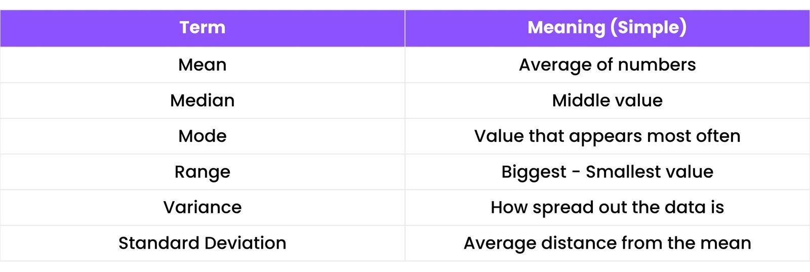
Example:
Let’s say student scores are:
[85, 90, 75, 95, 80]
- Mean = (85 + 90 + 75 + 95 + 80) / 5 = 85
- Median = 85 (middle value)
- Mode = No repeating value
- Range = 95 - 75 = 20
5.2 Probability Distributions
Probability shows how likely something is to happen. A probability distribution shows all possible outcomes and how likely each one is.
Types of Distributions:
1. Uniform Distribution
- All outcomes are equally likely.
Example: Rolling a dice (each number has 1/6 chance)
2. Normal Distribution
- Bell-shaped curve. Most values are around the mean.
Example: Heights of people, test scores.
import numpy as np
import matplotlib.pyplot as plt
data = np.random.normal(0, 1, 1000) # Mean 0, Std Dev 1, 1000 points
plt.hist(data, bins=30)
plt.title("Normal Distribution")
plt.show()
3. Binomial Distribution
- Used when there's only 2 outcomes like yes/no, success/failure.
Example: Tossing a coin 10 times.
5.3 Bayes’ Theorem
Bayes’ Theorem helps you update your belief when you get new information.
Formula:
$$P(A|B) = \frac{P(B|A) \times P(A)}{P(B)}$$
Where:
- $P(A|B)$ = Probability of A given B (updated belief)
- $P(B|A)$ = Probability of B given A (how likely B is if A is true)
- $P(A)$ = Probability of A happening
- $P(B)$ = Probability of B happening
Example:
Suppose:
- 1% of people have a disease ($P(\text{Disease}) = 0.01$)
- Test is 99% accurate
What is the chance a person really has the disease if they tested positive? Bayes' Theorem helps you solve this.
5.4 Hypothesis Testing
It helps you test if a claim about data is true or not using evidence.
Steps in Hypothesis Testing:
- State the Hypotheses:
- Null Hypothesis ($H_0$): Nothing is happening
- Alternative Hypothesis ($H_1$): Something is happening
- Choose Significance Level ($\alpha$):
- Usually 0.05 (means 5% risk of being wrong)
- Perform the Test:
- Use statistical test (like t-test, z-test)
- Compare p-value with $\alpha$:
- If p-value < $\alpha$ → Reject $H_0$ (significant result)
Example:
Claim: A new teaching method improves test scores.
You collect scores from students with old and new methods and compare. If p-value is small, you reject the null hypothesis and accept the new method works.
5.5 P-Values and Confidence Intervals
What is a p-value?
The p-value tells you how likely your results happened by random chance.
- Small p-value (< 0.05) = Result is significant (not by chance)
- Large p-value (> 0.05) = Result is likely due to chance
What is a Confidence Interval?
It tells you a range of values where you believe the true result lies — with confidence.
Example:
"Average height is 160 cm ± 5 cm with 95% confidence."
Means you are 95% sure that the real average height is between 155 cm and 165 cm.
6. EXPLORATORY DATA ANALYSIS (EDA)
EDA is the process of exploring and understanding your dataset before building any models. Think of it like looking at your data under a magnifying glass to:
- Spot patterns
- Find missing values
- Identify outliers
- Understand relationships between columns
6.1 Univariate, Bivariate, and Multivariate Analysis
Univariate Analysis
- "Uni" means one – so we analyze one column at a time
Goals:
- Understand the distribution of values
- Find mean, median, mode, min, max
- Detect outliers or skewness
Examples:
df["Age"].describe() # Basic statistics for 'Age' column
sns.histplot(df["Age"]) # Histogram to show age distribution
sns.histplot(df["Salary"]) # Histogram to show salary distribution
You might find:
- Most customers are aged 20–30
- Salaries are mostly between ₹20,000–₹50,000
Bivariate Analysis
- "Bi" means two – analyze two columns together
Goals:
- See relationships between variables
- Compare values using graphs
Examples:
sns.scatterplot(x="Age", y="Spending", data=df)
sns.boxplot(x="Gender", y="Spending", data=df)
You might learn:
- Older people spend more
- Males and females have different spending patterns
Multivariate Analysis
- Analyze three or more columns together
Goals:
- Understand how multiple factors interact
- Build a deeper picture
Examples:
sns.pairplot(df[["Age", "Salary", "Spending"]])
sns.heatmap(df.corr(), annot=True)
You might find:
- Salary and spending are highly related
- Age has little effect on salary
6.2 Outlier Detection
Outliers are data points that are very different from others. They can confuse your model if not handled properly.
Methods to detect outliers:
1. Boxplot
- Any dots outside the box are outliers.
sns.boxplot(y="Income", data=df)
2. Z-score
from scipy.stats import zscore
df["Z_Score_Income"] = np.abs(zscore(df["Income"]))
outliers = df[df["Z_Score_Income"] > 3]
3. IQR Method
Q1 = df["Income"].quantile(0.25)
Q3 = df["Income"].quantile(0.75)
IQR = Q3 - Q1
outliers_iqr = df[(df["Income"] < (Q1 - 1.5 * IQR)) | (df["Income"] > (Q3 + 1.5 * IQR))]
What to do with outliers?
- Keep them if they are important
- Remove them if they are errors
- Transform data (like log scale) to reduce their effect
6.3 Correlation Matrix
Correlation shows how strongly two columns are related.
Range: -1 to +1
- +1: Perfect positive correlation
- -1: Perfect negative correlation
- 0: No correlation
How to use it:
corr_matrix = df.corr()
sns.heatmap(corr_matrix, annot=True, cmap="coolwarm")
You can see:
- Which features move together (example: Salary and Experience)
- Which features are negatively related (example: Age and Screen Time)
6.4 Feature Engineering Techniques
Feature Engineering means creating new columns or modifying existing ones to help the model learn better.
Common Techniques:
1. Creating New Features
df["Age_Group"] = pd.cut(df["Age"], bins=[0, 18, 30, 45, 60, 100], labels=["Teen", "Young", "Adult", "Senior", "Old"])
2. Encoding Categorical Variables
df = pd.get_dummies(df, columns=["Gender", "City"])
3. Scaling Values
from sklearn.preprocessing import StandardScaler
scaler = StandardScaler()
df["Salary_scaled"] = scaler.fit_transform(df[["Salary"]])
4. Date Features
df["Year"] = df["Purchase_Date"].dt.year
df["Month"] = df["Purchase_Date"].dt.month
5. Interaction Features
df["Income_x_Age"] = df["Income"] * df["Age"]
7. MACHINE LEARNING BASICS
Machine Learning (ML) means teaching a computer to learn from data and make decisions or predictions — without being told what to do step by step.
7.1 Supervised vs Unsupervised Learning
Supervised Learning
- The model learns from labeled data.
- (We give the correct answers during training.)
Example:
If you give student scores along with their pass/fail status, the model learns to predict pass/fail for new students.
Data example:
Hours Studied | Score | Result
--------------------------------
    2         | 50    | Fail
    5         | 90    | Pass
Common Algorithms:
- Linear Regression
- Logistic Regression
- Decision Tree
- Random Forest
- K-Nearest Neighbors (KNN)
Unsupervised Learning
- The model learns from data without labels.
- (No correct answers are given — the model finds hidden patterns.)
Example:
Given only customer purchase data, the model groups similar customers together (like “high-spenders” or “frequent buyers”).
Data example:
Customer | Purchases | Visits
--------------------------------
A        | 1000      | 10
B        | 300       | 2
Common Algorithms:
- K-Means Clustering
- Hierarchical Clustering
- PCA (Principal Component Analysis)
7.2 Train/Test Split, Cross-Validation
Train/Test Split
Before training a model, we divide the data:
- Training Set → Used to teach the model
- Test Set → Used to check how well it learned
Usually:
- 80% data → training
- 20% data → testing
from sklearn.model_selection import train_test_split
X = df[['Hours_Studied']]
y = df['Result']
X_train, X_test, y_train, y_test = train_test_split(X, y, test_size=0.2)
Cross-Validation
- Instead of testing once, we test multiple times on different parts of data to get a better accuracy estimate.
- Cross-validation avoids bad luck from one bad test split.
from sklearn.model_selection import cross_val_score
scores = cross_val_score(model, X, y, cv=5) # 5-fold cross-validation
print(scores.mean())
7.3 Model Evaluation Metrics (Accuracy, Precision, Recall, F1-score)
Once the model gives predictions, we need to check how good it is.
Let’s assume we built a model to predict if an email is spam or not.
Accuracy
- Tells us how many total predictions were correct.
Example: If 90 out of 100 are right → accuracy = 90%
Accuracy = (Correct Predictions) / (Total Predictions)
But: Accuracy alone can mislead when data is imbalanced.
Precision
- Out of all emails the model predicted as spam, how many were actually spam?
Precision = TP / (TP + FP)
- TP: True Positive (correct spam prediction)
- FP: False Positive (wrongly predicted spam)
Recall
- Out of all actual spam emails, how many did we correctly find?
Recall = TP / (TP + FN)
- FN: False Negative (missed spam)
F1-Score
- F1-Score is a balance between Precision and Recall.
- When data is imbalanced, F1 is the best metric to use.
F1-Score = 2 * (Precision * Recall) / (Precision + Recall)
7.4 Overfitting vs Underfitting
Overfitting
- Model learns too much from training data, including the noise.
- Great on training set
- Bad on test set
Think of a student memorizing answers, but failing in real exams.
Underfitting
- Model doesn’t learn enough — too simple to understand the pattern.
- Bad on both training and test sets
Think of a student who didn’t study at all — just guesses randomly.
How to Fix?
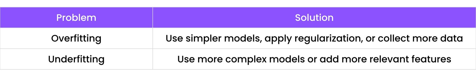
8. COMMON ML ALGORITHMS
These are the most widely used algorithms every beginner in data science should know. Each has its own use case, and the choice is based on:
- The type of data
- The problem to solve (e.g., prediction, classification, grouping)
8.1 Linear & Logistic Regression
Linear Regression
- Used when we want to predict a number (like marks, salary, price).
- It draws a straight line through the data points.
Example: Predicting marks based on hours studied.
Formula:
$$y = mx + c$$
Where:
- `y` is the output (predicted value)
- `x` is the input (feature)
- `m` is the slope (learned weight)
- `c` is the intercept
Logistic Regression
- Used when we want to predict a category (yes/no, spam/not spam, pass/fail).
- Even though it has “regression” in the name, it’s used for classification.
Example: Predicting if a student will pass or fail based on study hours.
8.2 Decision Trees & Random Forest
Decision Tree
- It splits the data into branches like a tree, based on questions.
Example:
- If Age > 18 → go right
- Else → go left
- ✅ Easy to understand
- ❌ Can overfit on small data
Random Forest
- Random Forest = many decision trees combined.
- It uses voting from multiple trees to give a better result.
- More accurate than a single tree
- Reduces overfitting
8.3 K-Nearest Neighbors (KNN)
- KNN looks at the ‘K’ closest points to a new data point and votes.
- If most nearby points are "Pass", then new data is also "Pass".
Example: Predicting if a new student will pass, based on how nearby students performed.
- ✅ Simple to understand
- ❌ Slow with large datasets
8.4 Support Vector Machines (SVM)
- SVM draws a line (or hyperplane) that best separates the data into classes.
- It tries to keep the widest possible margin between the two groups.
Example: Classifying if a message is spam or not spam.
- ✅ Works well in complex spaces
- ❌ Can be hard to tune
8.5 K-Means Clustering
- K-Means is an unsupervised learning algorithm.
- It groups data into K clusters based on similarity.
Example: Grouping customers based on purchase behavior.
- ✅ Easy to use
- ❌ You must choose the value of K
- ❌ Sensitive to outliers
8.6 Principal Component Analysis (PCA)
- PCA is a dimensionality reduction technique.
- It reduces many columns (features) into fewer important components, keeping the most useful information.
Why use PCA?
- To make models faster
- To remove noise
- To visualize high-dimensional data in 2D or 3D
- ✅ Makes big data easier to handle
- ✅ Helps in visualization
- ❌ May lose some information
9. SCIKIT-LEARN ESSENTIALS
Scikit-learn (or sklearn) is one of the most popular Python libraries for Machine Learning. It provides tools for:
- Data preprocessing
- Training models
- Evaluating models
- Improving models
...all in one place.
9.1 Preprocessing Pipelines
What is Preprocessing?
Before training a model, we must prepare the data. This includes:
- Handling missing values
- Scaling numbers
- Encoding text (like “Male”, “Female” → 0, 1)
What is a Pipeline?
- A Pipeline is a step-by-step process where you:
- Clean the data
- Scale or encode it
- Train the model
- Instead of writing multiple steps, you bundle them into one line.
Example:
from sklearn.pipeline import Pipeline
from sklearn.preprocessing import StandardScaler
from sklearn.linear_model import LogisticRegression

pipeline = Pipeline([
    ('scaler', StandardScaler()),
    ('logreg', LogisticRegression())
])
pipeline.fit(X_train, y_train)
Now `pipe` handles both scaling + model training in one go.
9.2 Model Training & Evaluation
Train a Model
from sklearn.linear_model import LogisticRegression
model = LogisticRegression()
model.fit(X_train, y_train)
Make Predictions
predictions = model.predict(X_test)
Evaluate the Model
from sklearn.metrics import accuracy_score
print(accuracy_score(y_test, predictions))
You can also use:
- `precision_score()`
- `recall_score()`
- `f1_score()`
9.3 Hyperparameter Tuning
What are Hyperparameters?
Hyperparameters are settings you choose before training a model.
Example:
- Number of trees in a Random Forest
- Value of K in KNN
- Learning rate in Gradient Boosting
Choosing the right hyperparameters can make a huge difference in model performance.
Example:
from sklearn.ensemble import RandomForestClassifier
model = RandomForestClassifier(n_estimators=100, max_depth=10)
Here, `n_estimators` and `max_depth` are hyperparameters.
9.4 Grid Search & Randomized Search
Grid Search
- Tests all possible combinations of hyperparameters.
- ✅ Finds the best
- ❌ Can be slow if combinations are many
from sklearn.model_selection import GridSearchCV
param_grid = {'n_estimators': [50, 100, 200], 'max_depth': [5, 10, None]}
grid_search = GridSearchCV(RandomForestClassifier(), param_grid, cv=5)
grid_search.fit(X_train, y_train)
print(grid_search.best_params_)
Randomized Search
- Tests random combinations of parameters, not all.
- ✅ Faster
- ✅ Good for large parameter spaces
- ❌ May miss the best if unlucky
from sklearn.model_selection import RandomizedSearchCV
from scipy.stats import randint
param_dist = {'n_estimators': randint(50, 200), 'max_depth': [5, 10, None]}
random_search = RandomizedSearchCV(RandomForestClassifier(), param_distributions=param_dist, n_iter=10, cv=5)
random_search.fit(X_train, y_train)
print(random_search.best_params_)
10. SQL FOR DATA SCIENCE
SQL (Structured Query Language) is used to talk to databases. As a Data Scientist, you use SQL to:
- Get data
- Filter it
- Summarize it
- Prepare it for analysis
Let’s break it down step-by-step.
10.1 Basic SELECT Statements
The `SELECT` statement is used to get data from a table.
Syntax:
SELECT column1, column2 FROM table_name;
Example:
SELECT Name, Age FROM Customers;
To get all columns, use `*`:
SELECT * FROM Products;
10.2 Filtering & Sorting
Filtering Rows (WHERE clause)
You use `WHERE` to choose only specific rows.
SELECT * FROM Orders WHERE Amount > 100;
You can also use:
- `=`, `!=`, `<`, `>`, `<=`, `>=`
- `AND`, `OR`, `NOT`
- `IN`, `BETWEEN`, `LIKE`
Example:
SELECT Name, City FROM Users WHERE Age >= 18 AND City = 'New York';
Sorting Rows (ORDER BY)
SELECT * FROM Employees ORDER BY Salary DESC;
- `ASC` = ascending (default)
- `DESC` = descending
10.3 Aggregation Functions
These functions summarize your data.
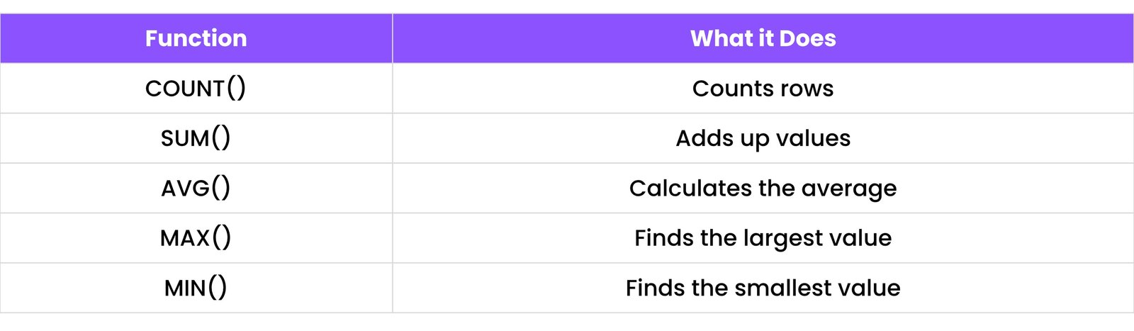
Example:
SELECT COUNT(OrderID), AVG(Price) FROM Products;
10.4 JOINS, GROUP BY, HAVING
JOINS
- Used to combine data from two or more tables.
Types of Joins:
- `INNER JOIN`: only matching rows
- `LEFT JOIN`: all from left + matches from right
- `RIGHT JOIN`: all from right + matches from left
- `FULL JOIN`: all from both sides
SELECT Orders.OrderID, Customers.CustomerName
FROM Orders
INNER JOIN Customers ON Orders.CustomerID = Customers.CustomerID;
GROUP BY
- Used to group rows that have the same value in a column.
SELECT Country, COUNT(CustomerID)
FROM Customers
GROUP BY Country;
HAVING
- Used to filter grouped data (like `WHERE` but for groups).
SELECT Country, COUNT(CustomerID)
FROM Customers
GROUP BY Country
HAVING COUNT(CustomerID) > 5;
10.5 Subqueries and Window Functions
Subqueries
- A query inside another query.
Example:
SELECT ProductName, Price
FROM Products
WHERE Price > (SELECT AVG(Price) FROM Products);
Window Functions
- Used to perform calculations across a set of rows without grouping.
Common Window Functions:
- `ROW_NUMBER()`
- `RANK()`
- `DENSE_RANK()`
- `SUM() OVER()`
Example:
SELECT
    EmployeeName,
    Department,
    Salary,
    RANK() OVER (PARTITION BY Department ORDER BY Salary DESC) as RankInDept
FROM Employees;
Here, employees are ranked within each department.
11. WORKING WITH REAL DATASETS
In Data Science, we often work with real-world datasets that come in many formats — like CSV, Excel, JSON, or even from websites and APIs. This chapter teaches you how to get, load, and explore real data in Python.
11.1 Loading CSV/Excel/JSON
Loading CSV (Comma-Separated Values):
- CSV files are the most common format used for datasets.
import pandas as pd
df = pd.read_csv("data.csv")
print(df.head())
You can also:
- Set a different separator: `pd.read_csv("file.txt", sep="\t")`
- Skip rows: `skiprows=1`
- Rename columns after loading
Loading Excel Files:
- Excel files can have multiple sheets.
- Make sure to install `openpyxl`:
# pip install openpyxl
df_excel = pd.read_excel("data.xlsx", sheet_name="Sheet1")
Loading JSON Files:
- JSON (JavaScript Object Notation) is used for structured data, often from web APIs.
import pandas as pd
df_json = pd.read_json("data.json")
If you get JSON from a URL:
import requests
import pandas as pd
url = "https://jsonplaceholder.typicode.com/todos/1"
response = requests.get(url)
data = response.json()
df_api = pd.DataFrame([data]) # Convert single JSON object to DataFrame
print(df_api)
11.2 Web Scraping Basics
Web scraping means collecting data from websites. Always check the website’s `robots.txt` file or terms of use before scraping.
Using BeautifulSoup:
import requests
from bs4 import BeautifulSoup

url = "http://example.com"
response = requests.get(url)
soup = BeautifulSoup(response.content, 'html.parser')
title = soup.find('h1').text
print(title)
You can scrape:
- Titles, prices, headlines, reviews, etc.
- Tables and lists
Make sure to install:
# pip install requests beautifulsoup4
11.3 APIs and JSON Handling
An API (Application Programming Interface) lets you ask for data from websites in a structured way, usually as JSON.
Example: Using a Public API
import requests
import json

url = "https://api.github.com/users/octocat"
response = requests.get(url)
data = response.json()
print(data["login"]) # Output: octocat
You can get:
- Weather data
- Stock prices
- Sports scores
- News headlines
Handling JSON in Python:
json_string = '{"name": "Alice", "age": 30}'
data_dict = json.loads(json_string) # Convert JSON string to Python dict
print(data_dict["name"]) # Output: Alice
You can also convert Python to JSON:
python_dict = {"city": "London", "population": 9000000}
json_output = json.dumps(python_dict, indent=4) # Convert dict to JSON string
print(json_output)
11.4 Open Datasets Resources
Here are some websites where you can download free datasets for learning:
12. TIME SERIES ANALYSIS
Time Series data means data collected over time — daily, monthly, yearly, etc.
Examples:
- Stock prices
- Weather data
- Website visits
- Electricity usage
12.1 DateTime Handling in Pandas
Pandas makes it easy to work with date and time.
Convert to DateTime:
import pandas as pd
df['Date'] = pd.to_datetime(df['Date_Column'])
Now you can:
- Sort by date
- Filter by month/year
- Group by time
- Extract parts of the date
df['Year'] = df['Date'].dt.year
df['Month'] = df['Date'].dt.month
Set date as index
df = df.set_index('Date')
Now you can resample, plot trends, and aggregate by time easily.
Resampling:
- Used to convert data from daily to monthly, weekly to yearly, etc.
monthly_sales = df['Sales'].resample('M').sum() # Sum sales by month
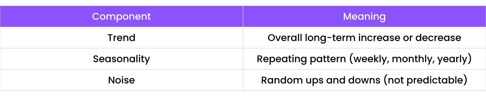
12.2 Trend, Seasonality, Noise
A Time Series has 3 key components:
Visualizing Components:
from statsmodels.tsa.seasonal import seasonal_decompose
result = seasonal_decompose(df['Value'], model='additive', period=12) # For monthly data
result.plot()
plt.show()
- `trend`: Shows overall direction
- `seasonal`: Repeats at regular interval
- `resid`: Noise or leftover data
12.3 Moving Averages
A Moving Average smooths the data by averaging values over a window. Helps to remove noise and highlight trends.
Simple Moving Average (SMA):
df['SMA_7'] = df['Sales'].rolling(window=7).mean()
This shows the 7-day average of sales.
Exponential Moving Average (EMA):
- Gives more weight to recent data.
- EMA reacts faster to recent changes.
df['EMA_7'] = df['Sales'].ewm(span=7, adjust=False).mean()
12.4 ARIMA Basics
ARIMA stands for:
- `AR` – Auto Regression (use past values)
- `I` – Integrated (make data stationary by differencing)
- `MA` – Moving Average (use past errors)
ARIMA Model
- Used to forecast future values in a time series.
Steps:
- Make the data stationary (no trend or seasonality)
- Find best (p, d, q) values:
- `p` = lag observations (AR part)
- `d` = differencing needed
- `q` = lagged forecast errors (MA part)
- Train ARIMA model
Example:
from statsmodels.tsa.arima.model import ARIMA

# Assuming 'data' is your time series
model = ARIMA(data, order=(5,1,0)) # Example order (p=5, d=1, q=0)
model_fit = model.fit()
forecast = model_fit.predict(start=len(data), end=len(data)+9) # Forecast next 10 points
print(forecast)
This gives the next 10 predicted values.
13. DEEP LEARNING INTRODUCTION
Deep Learning is a part of Machine Learning that uses artificial neural networks — computer systems inspired by how the human brain works. It’s used in tasks like:
- Image recognition
- Voice assistants
- Language translation
- Chatbots (like me!)
13.1 Neural Network Basics
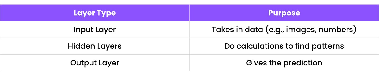
What is a Neural Network?
A neural network is made up of layers of nodes (neurons). Each neuron is connected to others and has a weight — just like how brain neurons pass signals.
How it works:
- Input data (like an image)
- Passes through layers of neurons
- Each neuron:
- Applies a function to inputs
- Sends output to next layer
- Final output is produced (like “Dog” or “Not Dog”)
13.2 Activation Functions
Activation functions decide whether a neuron should be “fired” (activated) or not. They add non-linearity — so the model can learn complex patterns.
Common Activation Functions:
- ReLU (Rectified Linear Unit): `max(0, x)`. Simple and widely used.
- Sigmoid: Squashes values between 0 and 1. Good for binary classification output layers.
- Softmax: Converts outputs to probabilities, summing to 1. Good for multi-class classification output layers.
- Tanh (Hyperbolic Tangent): Squashes values between -1 and 1.
Example (ReLU):
# In a neural network layer
# output = max(0, input * weight + bias)
Most deep learning models use ReLU in hidden layers.
13.3 Loss Functions
A loss function tells how far the prediction is from the truth. The model tries to minimize this loss while learning.
Common Loss Functions:
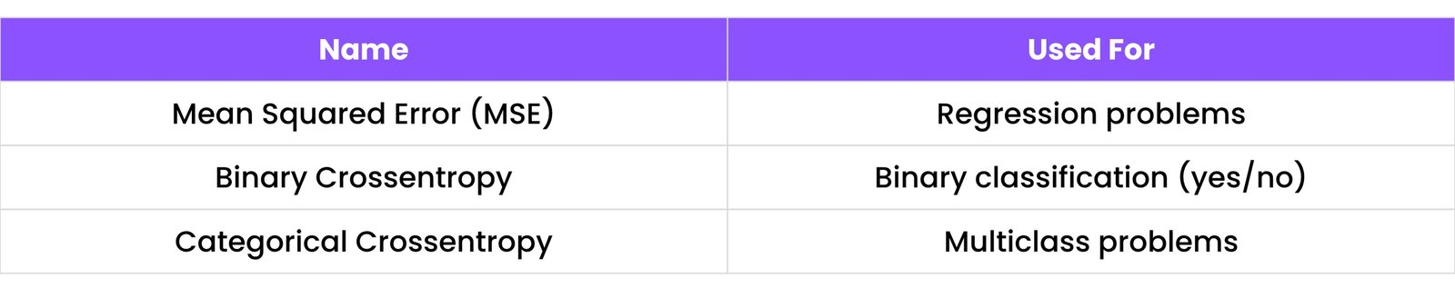
Example:
# For MSE:
# loss = (predicted_value - actual_value)**2
The model adjusts its weights to reduce the loss using an algorithm like gradient descent.
13.4 Introduction to TensorFlow & Keras
What is TensorFlow?
- TensorFlow is an open-source deep learning library developed by Google.
- It’s used to build, train, and deploy models — especially for big tasks like image or speech recognition.
What is Keras?
- Keras is a simple front-end to TensorFlow.
- It makes building models faster and easier, like a shortcut.
Example: Simple Neural Network in Keras:
from tensorflow import keras
from tensorflow.keras import layers

# 1. Define the model (a simple sequential model)
model = keras.Sequential([
    layers.Dense(units=64, activation='relu', input_shape=(10,)), # Input layer with 10 features
    layers.Dense(units=32, activation='relu'), # Hidden layer
    layers.Dense(units=1, activation='sigmoid') # Output layer for binary classification
])

# 2. Compile the model (configure for training)
model.compile(optimizer='adam',
              loss='binary_crossentropy',
              metrics=['accuracy'])

# 3. Train the model (using dummy data for example)
# X_train_dummy = ... (your training features)
# y_train_dummy = ... (your training labels)
# model.fit(X_train_dummy, y_train_dummy, epochs=10, batch_size=32)

# 4. Make predictions
# predictions = model.predict(X_test_dummy)

model.summary() # Prints a summary of the model architecture
- `Dense()` → creates a fully connected layer
- `relu`, `sigmoid` → activation functions
- `compile()` → sets optimizer & loss
- `fit()` → trains the model
14. PROJECTS AND PRACTICE IDEAS
Practicing projects is the best way to learn and grow in Data Science and Machine Learning. This chapter helps you understand:
- How to build a full ML project
- Where to get real-world datasets
- How to prepare for serious projects like capstones or Kaggle challenges
14.1 End-to-End ML Project Structure
A full ML project usually follows these 8 steps:
Step 1: Define the Problem
Example: "Can we predict house prices?"
Step 2: Collect the Data
Get data from:
- CSV/Excel files
- APIs
- Web scraping
- Open datasets
Step 3: Explore the Data (EDA)
Use charts and statistics to:
- Spot trends
- Find missing values
- Understand distributions
Step 4: Preprocess the Data
- Handle missing values
- Convert text to numbers
- Scale/normalize features
- Create new useful features
Step 5: Split the Data
Split into:
- Training set (80%)
- Test set (20%)
Step 6: Train Models
Try different algorithms:
- Logistic Regression
- Random Forest
- SVM, etc.
14.1 End-to-End ML Project Structure (continued)
Step 7: Evaluate Models
- Check accuracy, precision, recall, and F1-score.
- Use cross-validation.
Step 8: Improve and Deploy
- Tune hyperparameters
- Try ensemble models
- Deploy using tools like Flask, Streamlit, or cloud platforms
14.2 Kaggle Competitions
Kaggle is a popular platform for:
- ML competitions
- Datasets
- Notebooks (code examples)
- Learning resources
Beginner Competitions:
- Titanic: Predict survival
- House Prices: Predict house cost
- Digit Recognizer: Handwriting recognition
Each competition has:
- A dataset
- A leaderboard
- Public notebooks (to learn from others)
How to Start on Kaggle:
- Sign up at kaggle.com
- Go to "Competitions" → Select a beginner-level one
- Download the dataset
- Build a notebook using what you’ve learned
- Submit your predictions to see your rank
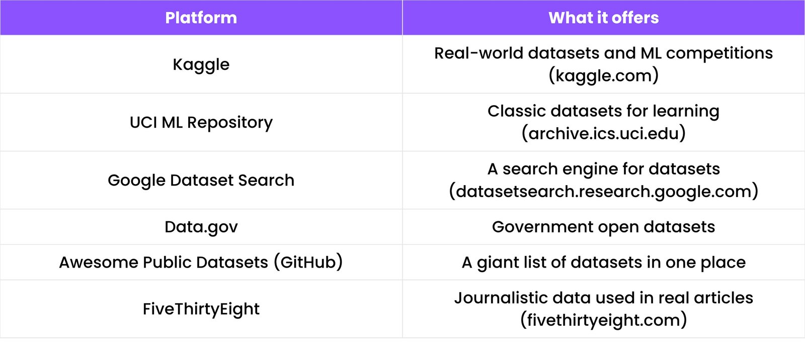
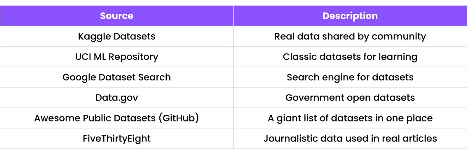
14.3 Real-world Dataset Sources
Here are some top places to find real datasets:
14.4 Capstone Project Tips
A capstone is a final project that combines everything you’ve learned.
Capstone Project Ideas:
- Predict customer churn for a telecom company
- Forecast sales for a store
- Sentiment analysis of movie or product reviews
- Classify whether a news article is real or fake
- Predict heart disease based on medical info
Tips for Success:
- Pick a topic you care about
- Use a real-world dataset
- It makes your project more impressive.
- Document everything clearly
- Write what you're doing and why.
- Visualize your results
- Use graphs, confusion matrix, feature importance, etc.
- Put it on GitHub
- Share your code and project for jobs or portfolio.
- Try deployment
- Use tools like Streamlit, Flask, or Gradio to turn your model into an app.
15. TOOLS & ENVIRONMENT
To work efficiently in Data Science, you need the right tools and setup. This chapter helps you understand:
- The most used environments
- Essential tools
- Shortcuts to boost your productivity
15.1 Jupyter Notebook Tips
What is Jupyter Notebook?
Jupyter Notebook is a web-based tool that lets you:
- Write code
- See outputs immediately
- Add notes and charts
Great for testing and exploring data
Basic Tips:
- Use `Shift + Enter` to run a cell
- Use `#` to add comments
- Use Markdown to write titles and notes
Useful Magic Commands:
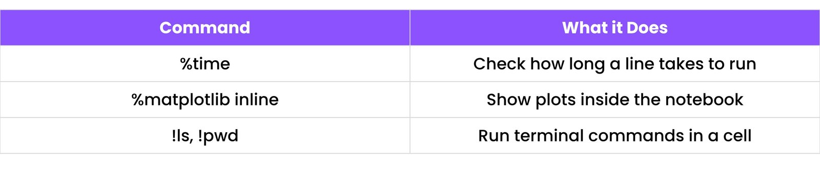
Auto-complete:
- Press `Tab` to auto-complete function names or see options.
Keyboard Shortcuts:
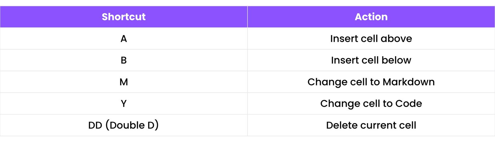
15.2 Git & GitHub for Data Science
What is Git?
- Git is a version control tool that helps you track changes in your code and projects.
What is GitHub?
- GitHub is a website to store and share your code using Git.
Perfect for:
- Saving progress
- Showing your projects to others
- Working with a team
Basic Git Commands:
git init # Start a new Git repo
git add . # Add all changes
git commit -m "Initial commit" # Save changes
git push origin main # Upload to GitHub
git pull # Download latest changes
Steps to Use GitHub:
- Create account on github.com
- Create a new repository
- Connect local folder using:
git remote add origin <your_repo_url>
git branch -M main
git push -u origin main
What to Upload:
- Jupyter notebooks
- CSV/Excel datasets
- ReadMe file to explain project
- Screenshots of results
15.3 Virtual Environments (venv, conda)
Why use virtual environments?
- Each project may need different versions of libraries.
- A virtual environment keeps them separate and avoids errors.
Using venv (built-in in Python)
python -m venv myenv # Create environment
source myenv/bin/activate # Activate (Linux/macOS)
# myenv\Scripts\activate # Activate (Windows Cmd)
Install packages in it:
pip install pandas numpy
Deactivate:
deactivate
Using conda (from Anaconda)
- Conda is a package manager and environment tool, widely used in data science.
conda create -n mydsenv python=3.9 # Create environment
conda activate mydsenv # Activate
conda install pandas numpy scikit-learn # Install packages
You can install tools like Jupyter, Scikit-learn, TensorFlow easily with:
conda install jupyter tensorflow
15.4 VS Code & Notebook Shortcuts
VS Code for Data Science
VS Code (Visual Studio Code) is a popular code editor that supports:
- Python
- Jupyter Notebooks
- GitHub integration
- Extensions for data science
Useful Extensions:
- Python (official by Microsoft)
- Jupyter
- GitLens
- Pylance (code suggestions)
- Material Theme (for better look)
VS Code Shortcuts:
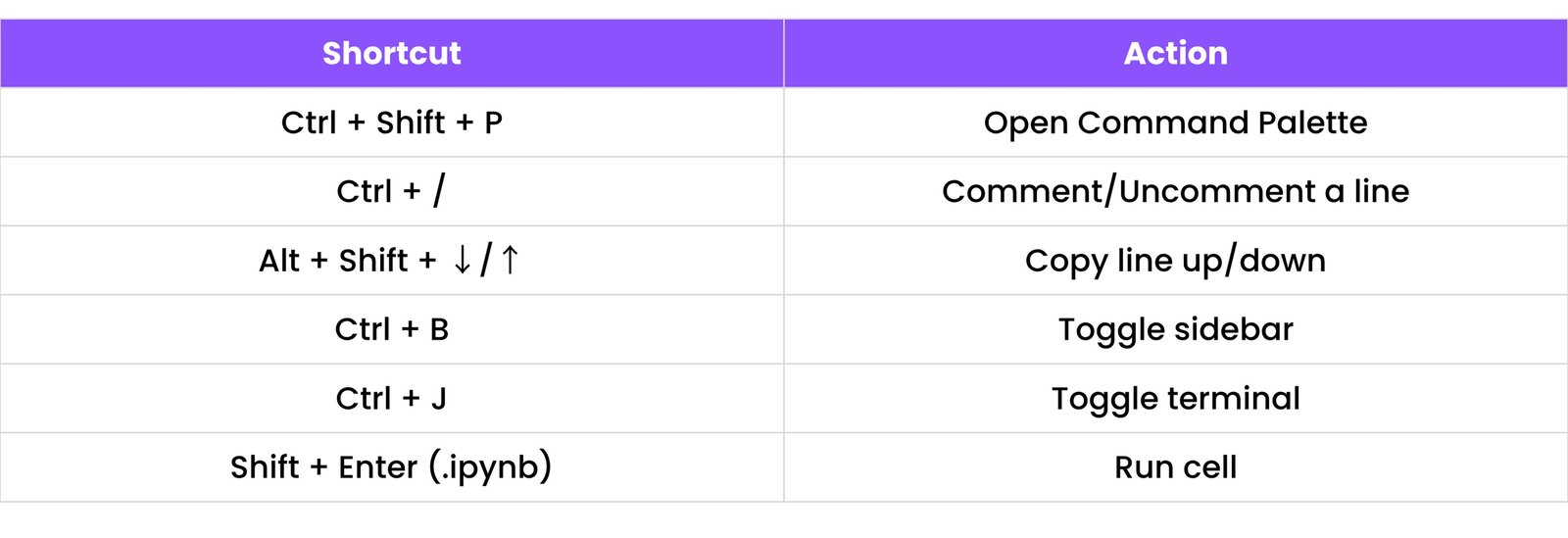
Run Jupyter Notebooks in VS Code:
- Open `.ipynb` file
- Use Run Cell button or `Shift + Enter`
- Outputs will appear right below the code
16. RESOURCES FOR LEARNING DATA SCIENCE
Whether you're just starting or want to go deeper, the right resources can speed up your learning and make it easier to stay motivated. This chapter lists trusted blogs, YouTube channels, courses, cheat sheets, and books that even a beginner can understand.
16.1 Blogs, YouTube Channels, and Courses
Top Blogs to Follow:

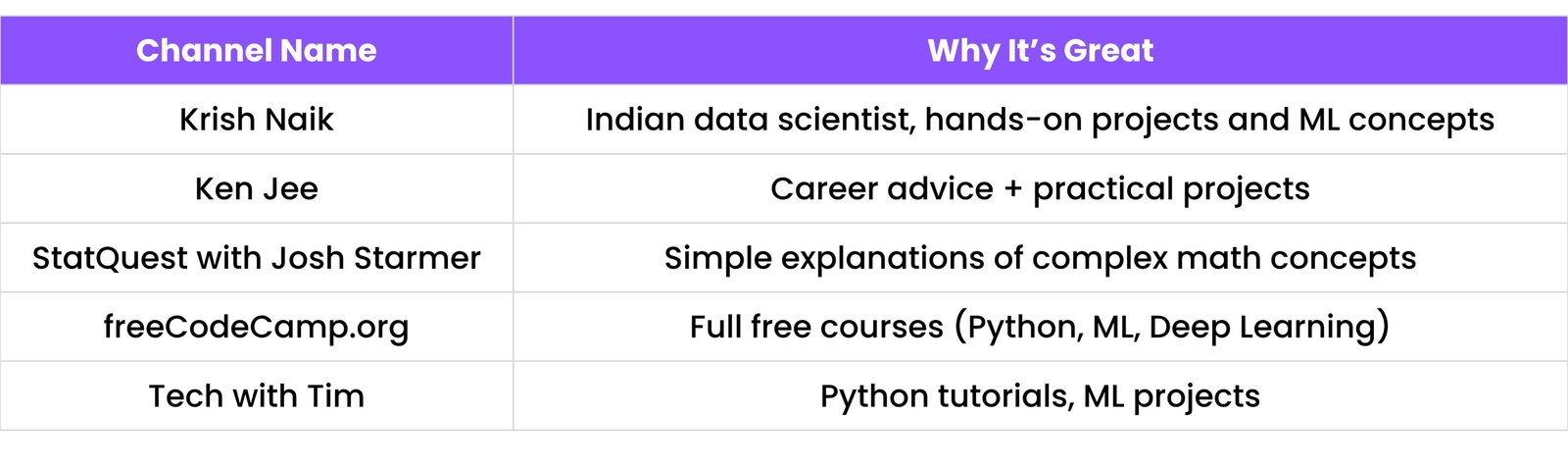
Best YouTube Channels:
Recommended Online Courses (Free & Paid):
- Coursera: Data Science Specialization by Johns Hopkins University
- edX: Professional Certificate in Data Science by HarvardX
- DataCamp: Interactive courses for Python, R, SQL
- Udemy: Python for Data Science and Machine Learning Bootcamp
- Google AI Education: Free courses and resources
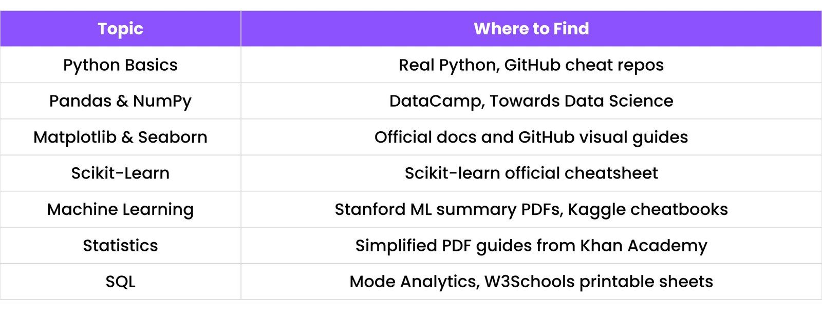
16.2 Cheat Sheets & PDF Summaries
Cheat sheets are quick reference guides that summarize important syntax and concepts.
Best Cheat Sheets for Beginners:
You can also make your own custom cheat sheets using tools like:
16.3 Books to Read
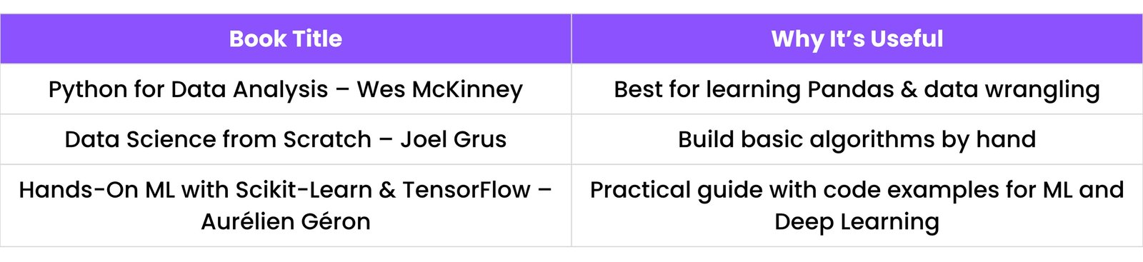
These books cover core concepts, real projects, and mathematical understanding — all in simple language.
Beginner-Friendly Books: